The Impact of Intranational Trade Barriers on Exports: Evidence from a Nationwide VAT Rebate Reform in China

The Impact of Intranational Trade Barriers

on Exports: Evidence from a Nationwide

VAT Rebate Reform in China

Jie Bai and Jiahua Liu

CID Faculty Working Paper No. 373

December 2019

and Fellows of Harvard College

at Harvard University

Center for International Development

Working Papers

The Impact of Intranational Trade Barriers on Exports:

Evidence from a Nationwide VAT Rebate Reform in China

Jie Bai Jiahua Liu

∗

December 13, 2019

Abstract

It is well known that various forms of non-tariﬀ trade barriers exist within a country.

Empirically, it is diﬃcult to measure these barriers as they can take many forms. We take

advantage of a nationwide VAT rebate policy reform in China as a natural experiment to

identify the existence of these intranational barriers due to local protectionism and study

the impact on exports and exporting ﬁrms. As a result of shifting tax rebate burden, the re-

form leads to a greater incentive of the provincial governments to block the domestic ﬂow of

non-local goods to local export intermediaries. We develop an open-economy heterogenous

ﬁrm model that incorporates multiple domestic regions and multiple exporting technologies,

including the intermediary sector. Consistent with the model’s predictions, we ﬁnd that ris-

ing local protectionism leads to a reduction in interprovincial trade, more “inward-looking”

sourcing behavior of local intermediaries, and a reduction in manufacturing exports. Anal-

ysis using micro ﬁrm-level data further shows that private companies with greater baseline

reliance on export intermediaries are more adversely aﬀected.

∗

Contact information: Bai: Harvard Kennedy School, e-mail: jie [email protected]ard.edu; Liu: Harvard Kennedy School,

email: jiahua [email protected]ard.edu. We thank Nikhil Agarwal, Pol Antras, Abhijit Banerjee, Panle Jia Barwick, Arnaud

Costinot, Dave Donaldson, Jack Feng, James Harrigan, Marc Melitz, Benjamin Olken, Gerard Padro, Robert Townsend,

Jeﬀery Wang, and lunch, seminar and conference participants at ASSA annual meeting, Cornell, Harvard, MIT, and

NEUDC for helpful discussions and comments. All errors are our own.

1 Introduction

“Aside from tariﬀ barriers (i.e., special charges levied at roadblocks), non-tariﬀ methods such as

physical barriers, outright prohibition, low-interest loans, and other ﬁnancial beneﬁts for commercial

establishments marketing local goods, ﬁnes for commercial establishments marketing nonlocal goods,

legal restrictions on price diﬀerences between local and nonlocal goods sold in commercial establishments,

local purchasing quotas, and administrative trivia (e.g

, medical, sanitation, epidemic prevention, product

quality, measurement, and other such licenses and certiﬁcates) were used to hamper trade in products

in a market economy.” (Young, 2000)

It is

well known that various forms of non-tariﬀ barriers exist within a country. While local governments

cannot block their borders or impose tariﬀs, their inﬂuence over the local regulatory apparatus can allow

them to impose signiﬁcant non-tariﬀ barriers to discourage non-local ﬁrms and non-local goods from

entering the local markets. Young (2000) gives many examples of such non-tariﬀ barriers in the Chinese

context. These barriers are especially likely to arise in countries’ where political and ﬁscal powers are

decentralized to subnational units. However, despite the general consensus on the existence of these local

trade barriers, we know relatively little about how costly they are in terms of real economic outcomes:

widespread interprovincial trade wars are very diﬀerent from occasional protectionist practices. What

makes this a challenging empirical problem to study is precisely the fact that these local barriers can

take many forms, and unlike tariﬀ barriers, they are diﬃcult to measure or even just to observe.

In this study, we take advantage of a nationwide VAT rebate policy reform in China in 2004 as a nat-

ural experiment to ﬁrst identify the existence of intranational trade barriers due to local protectionism

and then to quantify the impact on exports and ﬁrm performance. As a result of the shifting tax rebate

burden, the reform leads to a greater incentive of the provincial governments to block the domestic ﬂow

of non-local goods to local export intermediaries. By exploring a unique feature of the transaction-level

Chinese Customs Data that allows us to trace the sourcing locations of the export intermediaries, we

show that the intermediaries indeed become more “inward-looking” after the reform.

To go beyond the descriptive evidence and examine the impact on interprovincial trade and man-

ufacturing exports, we develop a theoretical model to guide the empirical analysis. The model is built

on the standard open-economy heterogeneous ﬁrm model by incorporating multiple domestic regions

and multiple exporting technologies, including the intermediary sector. We model the intermediary

technology following Ahn, Khandelwal, and Wei (2011), but with a new focus on the intermediary’s

role of domestic sourcing. The model predicts a fall in interprovincial trade (related to exporting via

intermediaries) and a reduction in manufacturing exports as a result of rising local protectionism.

To bring the theory to the data, we explore subnational variations in rebate burden and exposure

to the reform. First, for each province, we construct a measure of predicted rebate burden based on the

local intermediaries’ sourcing patterns prior to the reform and the tax rebate formula. Consistent with

the descriptive evidence, we ﬁnd that intermediaries located in provinces with a higher predicted rebate

burden become more “inward-looking” after the reform. Speciﬁcally, they source from fewer non-local

provinces and source a greater fraction of local goods. The results are robust to controlling for province

and time ﬁxed eﬀects, time-varying rebate rates, and province-speciﬁc time trends.

Using a diﬀerence-in-diﬀerence framework, we then examine the impact of increasing provincial

rebate burden on interprovincial trade ﬂows of indirect exports (i.e., exports via intermediaries). Our

estimate implies a trade elasticity of 1.2 with respect to provincial rebate burden. The magnitude is

comparable to existing estimates in the trade literature with respect to physical transportation costs,

indicating that political barriers can act as important frictions in hindering domestic trade.

Next, we examine the impact on manufacturing exports and manufacturing ﬁrms. To do so, we

construct a measure of reform exposure for each province-industry as the weighted average of the

predicted rebate burdens, where the weights are given by a province-industry’s baseline reliance on

intermediaries located in diﬀerent provinces. The results show that greater exposure to the reform

leads to reductions in both indirect exports as well as total exports. Using the NBS annual survey of

manufacturing ﬁrms, we show that, while some ﬁrms manage to switch to direct exporting, most of the

negative impact falls on private ﬁrms with a greater reliance on export intermediaries at baseline.

Last but not least, we explore the ﬁrm-level Customs data to shed light on local government behavior.

While systematic documentation of the protectionist practices does not exist, we ﬁnd suggestive evidence

that local governments may target large intermediaries, either due to limited administrative capacity or

ﬁxed costs of the intervention technology. However, beyond that, local oﬃcials do not appear to employ

additional local information in the targeting, such as an intermediary’s history of non-local purchase

and its product mix.

The study relates to the literature on domestic trade frictions. Ramondo, Rodr´ıguez-Clare, and

Sabor´ıo-Rodr´ıguez (2016) ﬁnd that domestic frictions are key to explaining the discrepancy between

standard trade models and the data. Costinot and Donaldson (2016) ﬁnd substantial gains from eco-

nomic integration among US agricultural markets from 1880-2002. More recent studies have quantiﬁed

domestic trade costs due to geographical barriers and poor transportation infrastructure (for example,

Limo and Venables (2001), Donaldson (2010), Banerjee, Duﬂo, and Qian (2012), and Faber (2014),

Anderson, Milot, and Yotov (2014), Atkin and Donaldson (2015), and Co¸sar and Fajgelbaum (2016)).

However, as discussed above, domestic trade barriers can take other forms. Lacking a good transporta-

tion network is responsible for the lack of greater economic integration, but it may not explain the full

story. Our ﬁndings show that political barriers imposed by local governments play an important role.

The paper also contributes to the literature on local protectionism (for example, Young (2000),

Naughton (2003), Bai, Du, Tao, and Tong (2004), Poncet (2003), Poncet (2005), and Holz (2009)).

There are two strands of this literature: the ﬁrst hinges on patterns of regional convergence as evidence

of rising protectionism (Young, 2000). However, a challenge with this approach is the lack of a theoretical

yardstick with which to evaluate the changes: reversal of ineﬃcient patterns of specialization can be

eﬃciency enhancing. The second strand of the literature relies on provincial input-output tables to

estimate the border eﬀect from a gravity equation (Poncet, 2005). The estimate may be confounded by

the presence of non-traded local goods and non-homothetic preferences.

We use micro ﬁrm-level data

to address some of the limitations and identify local trade barriers under relatively weak assumptions.

Our study is closely related and complementary to a concurrent paper by Barwick, Cao, and Li (2017),

in which the authors document local protectionism from “home bias” in passenger vehicle purchasing.

We focus on the supply side and study ﬁrms’ responses in light of rising local protectionism.

Finally, the study relates to the literature on resource misallocation. Institutions that distort the

eﬃcient allocation of resources can have a sizable eﬀect on economic outcomes. Hsieh and Klenow

(2009) estimate that the distortions in the Chinese economy reduce manufacturing productivity by 30%

to 50%. Brandt, Tombe, and Zhu (2013) estimate a large distortion on aggregate TFP due to ineﬃcient

factor inputs allocation within and between provinces in China. There has been a growing body of work

that tries to uncover particular sources of misallocation, including industrial policies and labor market

frictions (for example, Khandelwal, Schott, and Wei (2013), Fajgelbaum, Morales, Serrato, and Zidar

(2018) and Garicano, Lelarge, and Van Reenen (2016)). We show that local protectionism induced by

national tax policies can act as a potential source of resource misallocation.

The remainder of the paper is organized as follows. Section 2 describes the policy background.

Section 3 presents the model. Section 4 describes the data. Section 5 discusses the empirical strategy.

Section 6 presents the empirical results. Section 7 concludes.

Most of the studies rely on aggregate data. However, one limitation of the Chinese IO table is that it only reports a

net trade value, which aggregates the total net trade with the rest of China and the rest of the world. As a result, the

gravity equation estimates are also sensitive to functional form assumptions, including measures of distance between a

given province and the rest of China.

2 Background

2.1 Export Value-Added Tax Rebate Policy and the 2004 Reform

Value-added tax (VAT) is a general broad-based tax assessed on incremental value at each stage of the

production of goods and services. In China, the VAT rate is 17%, and it applies to most goods and

services that are bought or sold for use. The export tax rebate policy is such that the VAT paid for

exported goods can be refunded in whole or in part.

The idea is to remove taxes paid in all stages of

the production process so that the goods can enter the international markets without tax.

Under the

regime, when a manufacturer exports through an export intermediary (i.e., a foreign trade company,

or FTC), the FTC is entitled to a “Pay-First-and-Refund-Later” VAT refund treatment (Chan, 2008):

initially the FTC pays an output-tax-inclusive price to the manufacturer; after completing the export

transaction, the FTC can collect a partial or full refund of the tax paid earlier.

Prior to 2004, the central government was solely responsible for ﬁnancing the VAT rebates —

after completing an export transaction, an exporter ﬁrst receives its VAT refund from the provincial

government, which then receives the same amount of payment from the central government at the end

of each ﬁscal year. However, the rapid growth of exports after China entered the WTO in 2001 led

to a large backlog of rebate payments and put severe ﬁscal pressure on the central government. In

response to the mounting ﬁnancial burden, the central government implemented a major reform in 2004

The WTO Agreement on Subsidies and Countervailing Measures (SCM, Article 1.1a) allows members to provide

rebates on export duties as long as the rebate does not exceed the full extent of the duty imposed. Thus, in contrast to

other trade policies such as export subsidies, VAT rebates are sanctioned by the WTO.

In practice, the VAT rebates have remained incomplete for most commodities in China, and the rebate rates have been

adjusted over time as a policy tool to boost exports (Bai, Wang, and Zhong, 2011).

In general, the exact VAT rebate formula varies across diﬀerent business types. There are three VAT refund treatments

applied to diﬀerent types of exporters:

1. Pay-ﬁrst-and-refund-later: an exporter, typically a commercial enterprise, can have the VAT incurred during the

production process refunded in whole or in part prior to export. The refund rate could be lower than the VAT rate

charged. No tax burden is incurred if the refund rate equals to the VAT rate. This paper mainly analyzes the result

of a change to this treatment.

2. Exempt-credit-refund: an exporter, typically a production enterprise, will get refunded for the excess if the amount

of input VAT, from which the disallowed credit has already been deducted, is bigger than the VAT payable for the

current period. Exempt refers to the exemption of VAT for exports, and credit refers to the input VAT paid for the

purchase used in the manufacture of exports that will be oﬀset against the output VAT paid on local sales.

3. Tax exempt: an exporter, typically an export-processing enterprise, is not entitled to a VAT refund because either it

has not previously paid any input VAT on exports or it has paid input VAT but the refund policy is not applicable.

An example is bonded materials directly imported for use in export processing.

In general, a Chinese manufacturer can export through an FTC in two ways: either by simply selling the goods to the

FTC or by authorizing the FTC as an exporting agent (Wang, 2019). Before 2007, most manufacturer-FTC partnership

was in the form of the former, in which the “Pay-First-and-Refund-Later” treatment applies.

that shifted part of the rebate burden to the provincial governments.

In particular, the new policy

stipulates that, for the amount of rebates claimed by an exporter, the central government would ﬁnance

75% of the rebates, with the remaining 25% covered by the provincial government, depending on where

the exporter is located.

The justiﬁcation for the 75/25 sharing rule is that the VAT revenue is shared

between the central and provincial governments according to this ratio.

2.2 Rising Local Protectionism

While the reform alleviated the ﬁscal pressure on the central government, it created an unintended

consequence — it led to a strong incentive for provincial governments to discourage local FTCs from

servicing non-local manufacturers. Operating as export intermediaries, FTCs do not engage in man-

ufacturing activities but instead specialize in export services. They procure goods produced by other

manufacturing ﬁrms and resell them to the international markets after simple processing, such as re-

packaging and re-labeling. An FTC can source goods from manufacturers located in its own province or

from manufacturers located in other provinces. Under the post-reform rebate regime, for any non-local

goods sourced and exported by an FTC, the provincial government of the FTC has to ﬁnance 25% of

the VAT rebates despite the fact that it has not collected the VAT revenue share in the ﬁrst place,

which is paid to the provincial government where the manufacturer is located.

Figure 1 provides a graphical illustration. In this example, an upstream manufacturing ﬁrm produces

t-shirts worth 1000 USD. At the point of transaction between the manufacturer and the FTC, the latter

pays the former 1000 USD plus 17% VAT. The VAT revenue is split between the upstream province

and the central government. At the end of the transaction, the manufacturing ﬁrm issues a VAT invoice

to the FTC, with which the latter can get the tax refunded after exporting the t-shirts. Prior to the

reform, the entire rebates were ﬁnanced by the central government, but after the reform, the downstream

province where the FTC is located has to ﬁnance 25% of the rebates, even though it has not collected the

revenue share. This generates a large ﬁscal burden on the provinces where many FTCs are located. As

a result, the local governments have a strong incentive to block non-local goods, either by discouraging

the activities of the intermediary sector in general or by asking its local FTCs to divert more sourcing

toward local goods.

Note that the same reform also adjusted the rebate rates for many commodities across ﬁve distinct levels: 5%, 8%,

11%, 13%, and 17%, depending on the product category. In our empirical analysis, we collect detailed data on VAT rebate

rates and control for the concurrent changes across product sectors.

The sharing rule was later adjusted to 92.5/7.5 in 2005, in part due to the concerns over rising local protectionism

— see Section 2.2. Since 2015, it has completely reverted back to the original scheme, in which the central government

ﬁnances 100% of the rebates.

Media reports abound that the reform led to rising local protectionism in the ensuing years. Un-

fortunately, there has not been any systematic documentation of the protectionist measures introduced

by the local governments due to the illegal nature of such activities.

To understand the situation, we

conducted extensive research into media and government reports and interviewed a number of people

working in the intermediary sector. One speciﬁc protectionist measure stands out from these qualitative

accounts, which is through deliberate delays of VAT rebates for non-local goods: in particular, when

the local tax bureau receives a lot of VAT invoices for non-local goods ﬁled by an FTC, it could delay

the refund to the ﬁrm. There were many reports of such delays in VAT rebates in the early 2000s (for

example, Zhong (2004); Wen (2005); Wu (2004)).

Consistent with the above discussion, many FTCs became more “inward-looking” after the reform

to avoid delays in VAT rebates from their local governments. Figure 2 describes the changes in FTCs’

sourcing patterns before and after the reform. Panel A plots the cumulative distribution function of

the number of sourcing provinces among the FTCs in diﬀerent years. Panel B examines the fraction of

local goods in total export sales. We see that along both the extensive and intensive margins, the FTCs

had been becoming more outward-looking prior to the reform, but the trend sharply stopped in 2004.

While the time-series patterns are consistent with rising local protectionism, many macroeconomic

factors could be at play. Our empirical strategy controls for the aggregate shocks and explores within-

country across-province-industry and across-ﬁrm variations for identiﬁcation (see Section 5).

2.3 Impacts on Manufacturing Exports and Firm Performance

In light of the disruption of the FTCs’ domestic sourcing, upstream manufacturing ﬁrms could be ad-

versely aﬀected. Consider a typical manufacturing ﬁrm in China. The ﬁrm has two ways to export

its products to the international markets, either directly exporting on its own or indirectly exporting

through the FTCs.

Exporting through FTCs constitutes a signiﬁcant share of the total export activ-

ities in China. Figure 3 shows that a relatively small number of FTCs account for more than 30% of

the country’s total ordinary exports between 2001 and 2006. Figure A.1 shows that FTCs are respon-

sible for large fractions of exports in four major export industries, namely textiles, food products and

The Provisions on Prohibiting Regional Blockade in Market Economic Activities enacted in 2001 explicitly forbids

local governments from restricting ﬁrms, in any manner, to purchase only the products and inputs that are locally made.

The trend picked up again in 2006, which is consistent with the scaling down of the local rebate burden from 25% to

7.5%. In our empirical analysis, we take into account the revision of the sharing rule in constructing the policy shocks and

the results are robust to this adjustment.

There are two modes of indirect exporting via FTCs: the ﬁrst is through formal contracting and the second is direct

selling. The problem with the shifting tax rebate burden arises in the latter case; for the former, the rebate burden always

falls on the province where the manufacturing ﬁrm is located. Our study therefore focuses on the second case.

beverages, chemicals and chemical products, and electrical machinery and apparatuses.

Due to the high ﬁxed costs of direct exporting, many small and medium enterprises have relied on

FTCs to export (Lin, 2017). This is especially true for manufacturing ﬁrms located in inland provinces.

Panel A of Figure 4 shows the distribution of reliance on FTCs as deﬁned by the percentage of a

province’s total exports through FTCs. As the ﬁgure shows, many inland provinces heavily depend on

FTCs for exporting. On the other hand, most FTCs are located in the coastal areas, as shown in Panel

B of Figure 4.

As a result, small and medium manufacturers in inland regions may be particularly

susceptible to the protectionist practices that suppress non-local sourcing activities of the coastal FTCs.

In principle, the policy could also aﬀect downstream manufacturing ﬁrms that source production

inputs from non-local upstream ﬁrms. To fully characterize the impact on the domestic supply chain,

one would need information on ﬁrm-to-ﬁrm transactions. In this paper, we focus on the role of the

intermediary sector and the impact on upstream manufacturing ﬁrms by exploring a unique feature of

the Chinese Customs data that allows us to trace the sourcing locations of the FTCs. We describe the

data in more detail in Section 4.

In the next section, we develop a theoretical framework to formalize the discussion above and derive

testable predictions to guide our empirical analysis.

3 Theoretical Framework

The model extends the standard open-economy heterogeneous ﬁrm model in Melitz (2003) by adding an

intermediary sector. We model the intermediary technology following Ahn, Khandelwal, and Wei (2011)

but focus on its role in domestic sourcing and the result of impeding such activity. Importantly, we allow

for multiple intermediary technologies with diﬀerent costs of access, as well as heterogeneous reliance

on these technologies among diﬀerent provinces in China. This enables us to examine the diﬀerential

impact of increasing the costs of “indirect exporting” (i.e., exporting through intermediaries) due to

rising local protectionism on regions with diﬀerent baseline characteristics. The model generates several

reduced-form predictions that we bring to the data in the next section.

3.1 Basic Setup

Demand Side

Consider two countries, China and the Rest of the World (ROW), and two sectors, one diﬀerentiated-

Of the 31 provinces, 12 are classiﬁed as coastal provinces according to the oﬃcial Chinese deﬁnition: Beijing, Fujian,

Guangdong, Guangxi, Hainan, Hebei, Jiangsu, Liaoning, Shandong, Shanghai, Tianjin, and Zhejiang.

good sector and one numeraire-good sector. Consumers in both countries have Cobb-Douglas preferences

over the two sectors. In particular, foreign consumers’ utility can be written as:

U =

, α

+ α

= 1.

1 2

where A

and A

are the subutility obtained from numeraire good and diﬀerentiated good respectively.

Within the diﬀerentiated-good sector, consumers have CES preference over diﬀerent varieties ω:





 

σ−1 σ−1 σ−1

σ−1 σ−1

) A

= q(ω)

dω =

+ (X

)

ω∈Ω

where X

, for i, j ∈ {(C)hina, (R)OW }, represents the subutility derived from the consumption of

products made in i by consumers in j. Let P

denote the price index of Chinese export in the ROW:





= p

(ω)

1−σ

dω

1−σ

ω∈Ω

Thus, demand from the ROW for variety ω made in China is:



(ω)



−σ

(ω) =

Supply Side

Chinese consumers oﬀer one unit of labor and receive a normalized wage of 1 (assuming a freely traded

numeraire good produced by one unit of labor). Firms pay an entry cost of f

and draw productivity

φ from a Weibull distribution G(φ). Assuming constant marginal cost, the amount of labor required to

produce q units of output is l =

for a ﬁrm with productivity φ. The CES demand function implies that

 

1−σ

the optimal price for the domestic market is p

= The domestic proﬁts is π

(φ) =

ρφ

A Chinese ﬁrm can access the foreign market by directly exporting on its own or indirectly exporting

through an FTC. For direct exporting, the ﬁrm incurs a per period ﬁxed cost f

and a per unit

iceberg cost τ . For indirect exporting, the ﬁrm chooses among FTCs located in diﬀerent provinces.

Each province has a perfectly competitive intermediary sector consisting of identical FTCs open to all

provinces. If a ﬁrm φ of province i sells its variety through the intermediary sector in province j, it

ij ij

pays a ﬁxed cost f

and a per-unit variable cost γ

to the FTC but no longer incurs the iceberg cost.

Following Ahn, Khandelwal, and Wei (2011), we assume that the ﬁxed cost of indirect exporting is

lower than that of direct exporting, i.e., for any i and j, f

< f

3.2 Solving Firms’ Proﬁt Maximization Problem

The timing is as follows:

1. Entrants pays f

to enter the market and draw productivity φ. Low-productivity entrants exit.

2. Surviving ﬁrms make production and export decisions: ﬁrms choose to stay domestic or serve

both the domestic and foreign markets. Exporters decide on the exporting technology: direct or

indirect exporting, and if the latter, which FTC to use.

3. Prices and quantities are set.

We solve the ﬁrm’s problem backward:

Stage 3

Direct exporter φ solves the proﬁt-maximization problem

1 τ

(φ) = max π

(φ, p

) = p

q(p

) − q(p

)τ − f

⇒ p

(φ) =

φ ρφ

where p

is the price charged to foreign consumers. On the other hand, indirect exporter φ of province

i solves the problem:

∗

π (φ) = max π (φ, p

) = p

τq(τp

) − τq(τp

)γ − f ⇒ p (φ) =

I I I I I

φ ρφ

where province j

∗

is the proﬁt-maximizing FTC province for ﬁrm φ, and p (φ) is the price the ﬁrm

charges to the FTC in province j

∗

. Since the intermediary sector is perfectly competitive, it passes the

iceberg trade cost by setting the price in the foreign market as τ p

. The exporter has to sell to the FTC

quantity τq in order for quantity q to reach the foreign market.

Stage 2

Firms decide

whether to produce and export, and if export, which exporting technology to use. Following

the result above, the proﬁts from direct exporting is:

 

From now on, we abbreviate CR subscript for q

, R

, and P

1−σ

1 τ

(φ) = R − f

σ ρφP

∗

Similarly, the proﬁts of indirect exporting through the intermediary sector in province j is:

 

∗

Let π

= π , where j

∗

= argmax

π .

I I

Firms choose the optimal production and exporting technology by solving the following:

τγ

1−σ

π (φ) = R − f

I I

σ ρφP

π = max{π

+ π

, π

+ π

, π

Stage 1

Finally

, a ﬁrm of province m

decides whether to enter the market by calculating:

π(φ) = π(φ)dG(φ) − f

3.3 Solving for Productivity Cutoﬀs of Various Exporting Technologies

Suppose there are M provinces in China. Due to the variation in the ﬁxed and variable costs of

direct and indirect exporting technologies, for every province there is naturally a pecking order of

exporting technology, i.e., a productivity ladder that assigns ﬁrms with diﬀerent productivities into

diﬀerent optimal exporting technologies. Without loss of generality, suppose that for province i, the

productivity cutoﬀs of indirectly exporting through M provinces are ranked as φ

< φ

... < φ ,

I I I

where φ

denotes the productivity cutoﬀ of indirectly exporting through FTCs in province i

, the

mth province in the productivity ladder of province i.

This leads to an important observation that

m−1

> f and γ

< γ ∀m ∈ [2, M ].

We assume that own province has the lowest ﬁxed

I I I I

cost, and thus the own province is ranked at the last in the productivity cutoﬀ ladder, i.e., i = i

Furthermore, since f

> f

, ∀m and direct exporting incurs no additional variable cost, we have

< φ

, ∀m ∈ [1, M], where φ

denotes the productivity cutoﬀ of direct exporting.

Mathematically, there may be a province j that would not be economically viable for indirect exporting by province

ij ij

if there exists another province j

such that f > f and γ > γ . This can rationalize the empirical observations

I I I I

that a province never indirectly exports through another province. However, for tractability here we assume away such

provinces.

Suppose that for ﬁrms in province m, no two provinces have the same ﬁxed and variable costs of indirect exporting.

m−1

If f

> f and γ

> γ , then province i

would be strictly dominated by province i

m−1

, and vice versa;

I I I I

m−1

if f

< f and γ

> γ , then province i

m−1

would rank above i

in the productivity cutoﬀs of indirect

I I I I

exporting.

We can obtain φ

by setting the proﬁts of indirectly exporting through local province to zero:



(γ



)

1−σ

(φ

⇒ φ

) = 0, = A

I I I

We can also solve any φ

, m ∈ [2, M] from the indiﬀerence conditions:

 

(γ

)

1−σ

− (γ

m−1

)

1−σ

(φ

m−1

(φ

⇒ φ

I I

) = π ), = A

I I I I I

m−1

− f

I I

Finally, φ

can be obtained by equating the proﬁts of exporting directly and the proﬁts of exporting

indirectly through the highest ranked province in the productivity cutoﬀ ladder:

 

�



1−σ

where A = .

ρP σ

Figure A.3 illustrates the productivity cutoﬀs. One of the immediate implications from the discus-

sion above is that the most productive ﬁrms will be direct exporters, followed by indirect exporters,

and the least productive ﬁrms will serve domestic market only. We verify this pecking order in the

Chinese context: Figure A.4 plots the empirical TFP distribution of the three groups of ﬁrms, and the

patterns are largely consistent with the theoretical prediction, showing a rightward shift in productivity

distribution as we move from non-exporting ﬁrms to indirect and direct exporters.

1 − (γ

)

1−σ

(φ

) = π

(φ

), ⇒ φ

= A

1−σ

− f

3.4 Testable Predictions

After the policy reform, a greater fraction of the tax rebate burden falls on the provincial government,

leading to rising local protectionism that hinders the non-local sourcing activity of the intermediary

sector. To map the empirical context into the model, we consider an increase in the costs of indirect

exporting through non-local intermediaries; the bigger the rebate burden (proxying a local government’s

incentives to block non-local trade), the greater the increase. For simplicity, we assume that the cost

of the protectionist measures passes through the variable cost of indirect exporting. We state the

We follow Olley and Pakes (1996) and Brandt, Van Biesebroeck, Wang, and Zhang (2017) to estimate the TFP of

the Chinese manufacturing ﬁrms. The TFP used in the plot is demeaned by province and industry. Because the export

volume in the Customs Database is direct exports and that in the NBS survey is total exports, we deﬁne domestic ﬁrms as

the ones that have zero exports in both datasets, indirect exporters as the ﬁrms which have positive exports in the NBS

survey but zero exports in the Customs Database, and direct exporters as the ones whose share of direct exports among

total exports are more than 0.9 (∼ the 90th percentile in the sample).

assumption formally below:

Assumption 1. Let c denote a measure of the tax rebate burden falling on the provincial governments.

dγ dγ df

I I I

For any province i, > 0 if i

6= i, = 0 if i

= i, and = 0 ∀m ∈ [1, M],

dc dc dc

In principle, both the ﬁxed costs and variable costs of indirect exporting may be aﬀected. We derive

the predictions based on an increase in the variable costs, and all the results are qualitatively robust

for an increase in the ﬁxed costs.

Assumption 2.

= 0.

We abstract away from general equilibrium eﬀects and focus on partial equilibrium predictions. Our

reduced form analysis explores subnational variations in rebate burdens and exposures to the reform,

controlling for aggregate time shocks.

Below, we derive ﬁve predictions on Chinese ﬁrms’ exporting behavior as a result of the rebate

burden and an increase in the costs of indirect exporting. Details of the proofs are in Appendix C.

Prediction 1. The number and the export volume of direct exporters increase in c.

Plot (a) in Panel A of Figure 5 illustrates how the number and the export volume of direct exporters

respond in response to an increase in c. For province i, as c increases, the variable cost of indirect

exporting increases through every non-local province, including province i

, the highest province in the

productivity cutoﬀ ladder of indirect exporting. Therefore, some ﬁrms that were previously exporting

through the FTCs in province i

would switch to direct exporting, resulting in a leftward shift of the

productivity cutoﬀ of direct exporting φ

and an increase in the volume of direct exporting.

Prediction 2. For each province, the number of indirect exporters decreases in c. The indirect exporting

volume also decreases in c if the productivity cutoﬀs increase across all indirect exporting technologies.

As c increases, the proﬁts of indirect exporting through all provinces decrease, shifting up the

productivity cutoﬀ between staying domestic and indirect exporting. Combined with Prediction 1,

[φ

, φ

] shrinks and the number of indirect exporters decreases. However, the impact on the total

indirect exporting volume is theoretically ambiguous. This is because ﬁrms can switch to diﬀerent

provinces for indirect exporting after the reform, depending on how much more costly it becomes to

access an intermediary sector in a given province. It could be that a ﬁrm switches to a province with

higher ﬁxed cost but lower variable cost compared to what it has used before, in which case the ﬁrm’s

dγ

The theoretical results hold under a more general condition that > .

dc dc

(indirect) export volume would actually increase. On the other hand, if all the productivity cutoﬀs shift

to the right among the set of viable indirect exporting technologies, as illustrated in plot (b) in Panel

A of Figure 5, the indirect export volume would fall.

Next, we examine how domestic trade along diﬀerent indirect exporting routes, from manufacturing

ﬁrms in a given province to the intermediary sector in another province, is distorted. Let R

denote

the total indirect exporting volume ﬂowing from province i to its mth ranked FTC province in the

productivity cutoﬀ ladder prior to the reform:

m+1

= r

(φ)dG(φ).

After the reform, with an increasing local tax rebate burden, we can show that:

(1)

m+1

 

1−σ

m+1

∂R

∂r

(φ) τγ

�

∂Θ(φ ) ∂Θ(φ

)



I I I I I

= dG(φ) + R × −

∂c

∂c ρP ∂c ∂c

| {z }

Network eﬀect; ambiguous sign

Price eﬀect; ≤0

where Θ(φ) = φ

0σ−1

dG(φ

). This equation decomposes the eﬀect of increase in c on R

into two

−∞

parts: the price eﬀect and the network eﬀect. The price eﬀect captures the change in R

if indirect

exporters in i continue to export through the same provinces. The eﬀect channels through the eﬀect of

c on p

and the response of foreign demand to the change of prices. On the other hand, the network

eﬀect captures switchings among diﬀerent indirect exporting routes: indirect exporters of province i

may cease to export through province i

or they may shift more trade to i

, depending on how the

other routes are aﬀected. Panel B of Figure 5 illustrates the two eﬀects graphically. Given that it takes

time to look for new intermediaries and re-optimize among the indirect exporting routes, in the short

run, one may expect that the price eﬀect outweighs the network eﬀect, as shown in the case of Panel B.

Prediction 3. Given an increase in c, for any province i: (1) local exporters rely more on local FTCs

after the reform, i.e., the number and the export volume of indirect exports through local FTCs increase

in c; (2) the indirect export volume through other provinces decreases if the price eﬀect outweighs the

network eﬀect (as deﬁned in Equation (1)).

Finally, we examine heterogeneity across provinces based on their exposure to the reform, and map

these predictions to the data. Let B

denote the percentage change of the variable cost of indirectly

dγ

/dc

exporting from province i through j with respect to a change in c, i.e., B

. We can deﬁne a

A suﬃcient condition is that for any province i, dγ

/dc > dγ

/dc, ∀m, n s.t. γ

< γ

before the reform.

I I I I

province i’s exposure to the reform:

Deﬁnition 1. The exposure of province i to an increase in c, denoted as E

, is the sum of the percentage

change in variable costs of indirect exporting through all provinces from province i, weighted by the

share of indirect export volume through each province:

≡ B

, where =

I I

m∈[1,M]

n∈[1,M]

tuitively, a pro

vince is more “exposed” to the reform if it relies more on intermediaries in provinces

with larger increase in the variable cost of indirect exporting.

Prediction 4. If the price eﬀect is suﬃciently larger than the network eﬀect, given an increase in c,

indirect export volume from province i decreases more through provinces with larger B

Prediction 5. If the price eﬀect is suﬃciently larger than the network eﬀect, given an increase in c, a

province with higher exposure E will experience a larger percentage decrease in indirect exports.

4 Data

4.1 Chinese Customs Database

Our main data set is the Chinese Customs Database, which provides transaction-level trade ﬂows

information on the universe of China’s exports and imports. For this study, we focus on exports

during the time period between 2001 and 2006.

The data is collected and made available by the

Chinese Customs Oﬃce. For each transaction, we observe the exporting ﬁrm identity, ownership type

and location, trade type, value and quantity of the exports, 8-digit HS code, city in China where the

product is manufactured (i.e., the origin location), customs oﬃce where the transaction is processed

and the ﬁnal destination. The origin location information is a unique feature of the Chinese data that

is typically not present in other Customs databases. Conversations with oﬃcials from the Chinese

Customs oﬃce revealed that the collection of this information is required by the State Administration

of Taxation, for the purpose of cross-validating the VAT receipts for tax rebate.

To examine the behavior of FTCs, we follow the strategy in Manova and Zhang (2009) to identify

the set of FTCs based on Chinese characters that have the English-equivalent meaning of “importer”,

China entered WTO in 2001.The data after 2006 is no longer at the “transaction” level, and thus does not allow one

to identify the origin location of each export transaction.

“exporter”, and/or “trading” in their ﬁrm name.

This classiﬁcation is not perfect as there can be

both inclusion and exclusion errors.

As a ﬁrst pass, Figure A.2 plots the sourcing patterns of FTCs

and non-FTCs using the pooled data from 2000 to 2006. Reassuringly, we see that on average, FTCs

source from more provinces than non-FTCs. Not surprisingly, most (80%) non-FTCs export products

that come from a single province–the province in which the exporting ﬁrm is located. In other words,

these are manufacturing ﬁrms that produce and export on their own. Panel A of Table 1 presents the

summary statistics of FTCs in the pre-reform baseline year 2003.

4.2 NBS Survey of Manufacturing Firms

To examine the impact of local protectionism on manufacturing ﬁrm performance, we merge the Customs

data with the NBS annual survey of manufacturing ﬁrms.

The annual survey is conducted by the

National Bureau of Statistics (NBS), and it includes all industrial ﬁrms that are identiﬁed as being

either state-owned or non-state ﬁrms with sales revenue above 5 million RMB. As discussed in Brandt,

Biesebroeck, and Zhang (2012), even though a large number of ﬁrms (80%) are excluded from the

sample, they account for only a small fraction (9.3%) of the total economic activities in China.

Panel

B of Table 1 presents the summary statistics of the balanced sample of manufacturing ﬁrms (i.e., 57,301

ﬁrms that appear in all 6 years in the data from 2001 to 2006).

One important variable in the NBS data is a ﬁrm’s total export revenue. Compared to the export

sales captured in the Customs data, which only reﬂects a ﬁrm’s direct exports, the self-reported amount

in the NBS data presumably captures both direct exports and indirect exports through FTCs. In

principle, we can derive a ﬁrm’s indirect export revenue by subtracting the two numbers. One concern

with this approach is reporting noise, especially if ﬁrms consider some of their sales to FTCs as domestic

sales rather than “exports”. We address this concern in our empirical analysis (see Section 6.4).

In pinyin (Romanized Chinese), these phrases are: jin4chu1kou3, jing1mao4, mao4yi4, ke1mao4 and wai4jing1.

As noted in Khandelwal, Schott, and Wei (2013), some state-owned manufacturers may export through trading arms

of their production facilities under a name that contains phrases such as importer, exporter and trader.

We follow the standard procedure and link ﬁrms by their names following Yu and Tian (2012). We improve on the

previous procedure by ﬁrst standardizing ﬁrm names in both datasets.

Trade in services accounts for a small fraction of the total trade activities during this period. We follow the industry

concordance constructed by Brandt, Biesebroeck, and Zhang (2012) to ensure a coherent classiﬁcation over time.

There is a sharp increase in the number of ﬁrms in the sample between 2003 and 2004 as a result of the 2004 Industrial

census—many ﬁrms above the 5 million RMB cutoﬀ should have been in the sample in earlier years, but had been left

out due to issues with the business registry. To avoid the composition change, we focus on a balanced sample of ﬁrms. A

comparison between the balanced sample and the unbalanced sample can be found in Table B.1.

4.3 Export VAT Rebate Rates

We compile a comprehensive list of export VAT rebate rates at 10-digit HS product code from 2001 to

2006 based on oﬃcial announcements released by the Chinese government.

We aggregate the rebate

rates to 6-digit HS code by taking arithmetic averages (rebate rates within a 6-digit code are usually

identical). Panel C of Table 1 describes the distribution of rebate rates across 6-digit HS industries

in 2003. Over 80% of goods have a rebate rate of 13%; others categories include 0%, 5%, 10%, and

17% (full rebate). Section 5.1 describes how we use the rebate rates to construct measures of predicted

rebate burden for local governments under the new policy.

4.4 Provincial Statistical Yearbooks

The Provincial Statistical Yearbooks provide basic macroeconomic statistics for 31 provinces in mainland

China. Panel D of Table 1 presents basic summary statistics for the year 2003. We use information on

government revenue and expenditures to construct various proxies for local ﬁscal capacity. We expect

that the higher the predicted rebate burden as a share of local ﬁscal capacity, the stronger the incentive

of the local government to discourage non-local sourcing to alleviate the rebate burden.

5 Empirical Strategy

This section describes the empirical strategy to test the predictions in Section 3. We focus on Prediction

4 and 5, which guide us to exploit subnational variations and employ a diﬀerence-in-diﬀerence strategy

for identiﬁcation. Section 5.1 and 5.2 describe how we measure the rebate burden and exposure to

reform. Section 5.3 describes the empirical speciﬁcations for examining the impact on interprovincial

trade, sourcing patterns of FTCs, and exporting activities of manufacturing ﬁrms.

5.1 Predicted Rebate Burden

For each province, we compute a measure of predicted rebate burden based on local intermediaries’

pre-reform trading patterns and rebate rates across industries. Speciﬁcally, we calculate the amount of

VAT rebates each province would have to pay out due to its local FTCs’ non-local businesses for each

Export VAT rebate rates are published on the government website http://www.gov.cn/fuwu/chaxun/cktsl.html.

One caveat is that certain extra-budgetary sources of revenue are oﬀ the book (for example, money from selling lands,

which is known to be an important source of revenue for local governments in China). However, such information has

been poorly documented. To the extent that the diﬀerent sources of revenue may be correlated, we perform a series of

robustness checks using various measures that are available.

post-reform year had the non-local trading volume stayed the same as the pre-reform period. We scale

the predicted rebate amount by a province’s ﬁscal capacity, measured by total government revenue, to

capture the degree of ﬁscal stress induced by the policy change.

Formally,

P P

s∈S

0.25 × ι

× R

i=j

I,s

= , for t ≥ 2004

where s is 6-digit HS code and S is the universe of export products

; ι

is the VAT rebate rate of sector

s in year t; R is the sum of average indirect export volume from other provinces through j for

the three years before the reform; G

indicates the average total government revenue of province j in

the pre-reform period. 0.25 is the rebate share borne by the provincial government after the reform.

I,s

= 0 for t < 2004.

Conceptually, we expect that the higher predicted rebate burden would lead to a stronger incentive

to discourage non-local sourcing and consequently to greater costs of accessing the local intermediary

sector. Therefore, is a reduced-form way of capturing the cost shocks to the indirect exporting

dγ

/dc

technology as a result of increasing c, mapping to B

in the model.

Table 2 shows substantial variations across Chinese provinces in terms of the predicted rebate

burden.

An important part of the heterogeneity is coming from variations in baseline sourcing patterns

of the local FTCs, particularly the average non-locally sourced exports between 2001 and 2003.

5.2 Exposure to Reform

Next, we use the predicted rebate burden to construct a measure of reform exposure for each province.

The idea is that a province that relies more on FTCs in provinces with larger predicted rebate burden

would be more exposed to the reform in light of the greater protectionist incentives of other provinces.

Mathematically, following Deﬁnition 1 in the model, we construct the exposure measure as weighted

sum of the rebate burden:

= ˆ

m∈[1,M]

(2)

In the robustness checks, we consider alternative measures of ﬁscal capacity, including total tax revenue, VAT revenue,

and rollover balance, and obtain very similar results.

Throughout the paper, we use s to denote 6-digit HS code, S 2-digit HS code, and S the universe of export products.

There was a subsequent revision of the sharing rule after 2005, which changed the rebate share falling on the provincial

government to 0.075. In the robustness checks, we take into account the subsequent revision of the policy in constructing

the predicted rebate burden.

The complete list of predicted burdens in 2004 for each province can be found in Table B.2.

where ωˆ

the average pre-reform share of indirect export volume of province i through

. It captures i’s baseline reliance on export intermediaries in other provinces.

Table 2 shows meaningful variations in reform exposure across provinces.

This is primarily driven

by heterogeneity in indirect exporting choices at baseline. Figure 6 illustrates the cases for four provinces:

two northern provinces, Shanxi and Qinghai, and two southern provinces, Jiangxi and Hunan. For the

two northern provinces, most of their indirect exports in 2003 were through FTCs in the northern

coastal provinces. The opposite is true for the two southern provinces, suggesting that distance matters

for domestic trade.

Analogously, we can deﬁne the exposure measure at province-industry (2-digit HS code) level:

= ˆ

I,S

m∈[1,M]

where ωˆ

I,S

is the average pre-reform share of indirect exports of industry S in province i

I,S

that are through the intermediary sector of i

. This allows us to exploit ﬁner subnational variations

for identiﬁcation. We now turn to describe our empirical speciﬁcations in detail.

5.3 Empirical Speciﬁcations

5.3.1 Impact on Interprovincial Trade

Prediction 4 says that indirect export volume from province i would decrease more through provinces

with larger rebate burden. To examine this, we look at interprovincial trade ﬂows and exploit hetero-

geneity in the predicted rebate burden of the downstream province:

(3)

R = α + β

+ ν

+ λ

+ κ

Year + κ

Year + θ

+ θ

+ 

ijt

The dependent variable is the total amount of indirect exports that originated from province i and were

exported through FTCs in province j. The key regressor is j’s predicted rebate burden in year t. Our

baseline regression controls for province-pair FE ν

, year FE λ

, and province-speciﬁc linear time trends

for both provinces. Standard errors are clustered at the province-pair level.

This corresponds to a diﬀerence-in-diﬀerence speciﬁcation. The key assumption for identiﬁcation is

that without the reform, the average change in export volume would have been the same across each

The complete list of exposure measures in 2004 for each province can be found in Table B.2.

indirect exporting route. To examine this assumption, we check the correlations between the predicted

rebate burden with a rich set of provincial pre-reform characteristics, both in terms of the baseline level

and the growth rate.

The results, shown in Table B.3, are reassuring. Our main results in Section 6

are robust to controlling for these variables and their interactions with time (not shown).

One potential confounding factor is changing industrial rebate rates over time, which may be cor-

related with both the predicted rebate burden and the volume of indirect trade. To address this, we

further control for the average rebate rates faced by provinces i and j given their baseline export mix,

denoted as ι

and ι

in Equation (3).

5.3.2 Impact on the Sourcing Patterns of FTCs

direct implication of Prediction 4 is that FTCs in provinces with a greater rebate burden would

become more “inward-looking” in terms of their sourcing behavior. To examine this, we run the following

diﬀerence-in-diﬀerence regression at the ﬁrm level:

(4)

= α + β B

+ ν

+ λ

+ κ

Year + θι

+ 

where the outcome variables include exports sourced from local and non-local manufacturers, as well

as the share of exports sourced from local manufacturers by FTC f of province j at year t. The key

regressor of interest is B , the predicted rebate burden of province j in which f is located. We control

for ﬁrm FE ν

, year FE λ

, province-speciﬁc linear time trends, and the average rebate rate faced by

. Standard errors are clustered at the province level.

The variables we examine include the baseline levels and the growth rates of provincial government revenue, balance,

tax revenue, value-added tax, GDP, population and the baseline levels of total provincial exports, direct exports, indirect

exports, number of FTCs, and number of exporting ﬁrms.

The average rebate rate faced by province i is constructed as the average rebate rates of industries weighted by their

pre-reform value shares in the total exports the province manufactures:

01−03

i’s total exports of s

= ι

× .

s∈S

i’s total exports

01−03

The average rebate rate faced by province j is constructed as the average rebate rates of industries weighted by their

pre-reform value shares in total indirect exports through j:

= ι

P P

s∈S

v∈S i

In total, there are 31 provinces. All the main results in Section 6 are robust to using bootstrapped standard errors.

5.3.3 Impact on Manufacturing Exports

To examine the impact of local protectionism on manufacturing exports, we test Prediction 5 by using

the empirical exposure measure E

described in Section 5.2:

(5) Y

= α + β E

+ ν

+ µ

+ λ

+ κ

Year + θι

iSt

+ 

iSt

where the outcome variables include total exports and indirect exports originated from province-industry

iS in year t. The regression controls for province FE, industry FE, year FE, and province-speciﬁc linear

time trend. As discussed above, we further control for the time-varying average rebate rate at the

province-industry level.

Standard errors are clustered at the province level.

The identiﬁcation assumption is that without the reform, the average change in export volume would

have been the same across each province or province-industry. Table B.4 examines the correlations

between the province-level exposure measure with a rich set of provincial pre-reform characteristics,

both in terms of the baseline level and the growth rate. The main results in Section 6 are robust to

controlling for these variables and their interactions with time (not shown).

5.3.4 Impact

on Manufacturing Firms

Finally,

we examine the impact on manufacturing ﬁrms in terms of their performance and exporting

behavior using the ﬁrm-level annual NBS survey data. As discussed in Section 4.2, we can compute a

ﬁrm’s indirect exporting volume by comparing the export revenue reported in the NBS data and that

registered in the Customs data. Using this information, we can measure a ﬁrm’s baseline reliance on

indirect exports, IndirectDependence, as the fraction of indirect exports over total exports in the pre-

reform period. We focus on the sample of manufacturing ﬁrms with positive export volume at baseline

(either direct or indirect). A simple diﬀerence-in-diﬀerence regression examines the diﬀerential impact

of the reform on ﬁrms with varying degrees of baseline reliance on indirect exports:

φt

= α + βIndirectDependence

× Post

+ ν

+ λ

+ κ

Year + θι

+ 

φt

(6)

The average rebate rate of industry S (2-digit HS) in province i at year t is constructed analogously to ι

in Footnote

32 as the average rebate rates of exports weighted by the pre-reform value share in total exports of industry S in province

i :

01−03

i’s total exporexportst of s

iSt

= ι

× .

s∈S

i’s total exports of S

01−03

When the dependent variable is total exports, we modify the empirical exposure measure to more closely capture the

reform’s potential eﬀect on total exports. In particular, the weight in Equation (2) becomes the pre-reform value share of

indirect exports over total exports.

φt

= α + β

IndirectDependence

+ β

+ ν

+ λ

+ κ

Year + θι

ist

+ 

φt

where the outcome variables include direct and indirect export revenue, dummies for direct and indirect

exporting, and total sales (including domestic sales) of ﬁrm φ in province i at year t. The key regressor

is the interaction between ﬁrm φ’s baseline reliance on indirect exports and the post-reform dummy,

which equals to 1 for t ≥ 2004. λ

and ν

are year and ﬁrm ﬁxed eﬀects. The regression further controls

for the province-speciﬁc linear time trend and average rebate rate. Standard errors are clustered at the

province level.

We could replace the post-reform dummy with the reform exposure measure:

(7)

The

same framework also allows us to examine the heterogeneous impact across diﬀerent types of

ﬁrms. In light of a negative shock on the indirect exporting technology, ﬁrms that face greater challenges

of switching to direct export would be more adversely aﬀected. We examine the heterogeneity across

ﬁrms in Section 6.4. Last but not least, as discussed in Section 4.2, one caveat of the IndirectDependence

measure is that ﬁrms may not report all indirect exports in the NBS survey. In other words, some of the

“non-exporters” in the NBS data could well export through FTCs. We return to this point in Section

6.4 after presenting the main results.

6 Results

6.1 Impact on Interprovincial Trade

We begin by examining the impact of increasing provincial rebate burden on interprovincial trade ﬂows

of indirect exports, following the empirical speciﬁcation in Equation (3).

Results are shown in Table 3. Columns 1 and 2 show that increasing the predicted burden of a

province reduces the amount of indirect exports from other provinces, consistent with Prediction 4.

At the same time, the value share of indirect exports from other provinces via the local intermediary

sector decreases, as shown in Columns 3 and 4, and so does the number of FTCs engaging in non-

local sourcing, as shown in Columns 5 and 6. Based on the coeﬃcient estimate in Column 2, we

can compute the elasticity of interprovincial trade ﬂows of indirect exports with respect to provincial

rebate burden, which equals to 1.15.

This implies that an increase in a province’s rebate share from

Given that the indirect exports dependent variable in Section 5.3.1 is under inverse hyperbolic sine transformation,

√

the elasticity is calculated as ξ = β × B

× ≈ βB

. We use the 2004 provincial average predicted burden as an

empirical equivalent for B

25% to 30% would lead to a reduction of 23% of indirect exports from other provinces through the

local intermediary sector.

The magnitude is around 30% of existing elasticity estimates in the trade

literature with respect to physical transportation costs, suggesting that political barriers due to local

protectionism can act as important frictions in domestic trade.

Table B.5 shows the results using alternative measures of predicted burden. Table B.6 measures

predicted rebate burden accounting for the revision of the sharing rule in 2005. The results are robust.

6.2 Impact on the Sourcing Patterns of FTCs

Next, we examine how increasing provincial rebate burden aﬀects the sourcing patterns of the FTCs.

Table 4 presents the results following the empirical speciﬁcation in Equation (4). Consistent with the

results at the interprovincial level, Columns 1 and 2 show that increasing rebate burden decreases the

volume of indirect exports from non-local manufacturers. The magnitude of the estimated coeﬃcient in

Column 2 implies that increasing local rebate share from 25% to 30% would decrease a local FTC’s non-

local sourcing by 12%.

This captures the intensive-margin eﬀect, i.e., conditioning on still engaging

in non-local sourcing, comparing to the 23% reduction of total non-local indirect exports in Section 6.1,

which captures both the intensive-margin and extensive-margin eﬀects.

Columns 3 and 4 examine the impact on local goods. While negative, the impact is much less

pronounced compared to non-local goods (Column 4 versus Column 2). Together, these results imply

that the FTCs become more inward-looking after the reform: the share of local goods increases as ﬁrms

shift their sourcing activities away from non-local manufacturers, as shown in Columns 5 and 6.

The results using diﬀerent measures of the predicted rebate burden are presented in Table B.7 and

Table B.8. The results are robust to the alternative deﬁnitions.

6.3 Impact on Manufacturing Exports

Given that exporting through non-local FTCs constitutes an important exporting channel for Chinese

manufacturers (Figure 4), we next turn to examine the impact of increasing local trade barriers on man-

ufacturing exports, exploiting variations in the exposure to the reform across provinces and industries.

Table 5 shows the regression results, following the speciﬁcation in Equation (5). Columns 1 and

2 show that exports of a province-industry is negatively aﬀected by its exposure to the reform. The

Using the estimated elasticity, we can compute the eﬀect as (

0.3−0.25

× 100%) ×

ξ = −23%.

0.25

Recent papers such as Bernard, Eaton, Jensen, and Kortum (2003) and Eaton, Kortum, and Kramarz (2011) use

ﬁrm-level data and estimate trade elasticity in the range of 3.6 to 4.8.

The calculation follows the same procedure explained in Footnote 36 and 37.

magnitude of the estimated coeﬃcients implies that increasing the VAT rebate share from 25% to 30%

would decrease total exports of a given province-industry by 4% and decrease indirect exports by 6%.

Results using alternative exposure measures (based on diﬀerent measures of predicted rebate burden)

are presented in Table B.9 and Table B.10. Results are robust.

6.4 Impact on Manufacturing Firms

Finally, we delve into the level of individual manufacturers and examine how their production and

exporting activities are aﬀected by the reform based on their reliance on indirect exporting prior to the

reform. We focus on the sample of exporting ﬁrms at baseline.

Columns 1 and 2 of Table 6 report

the regression results of estimating Equations (6) and (7). The results indicate a substitution pattern

from indirect export to direct export among Chinese manufacturers after the reform.

The coeﬃcient

estimates in Panel A imply that, with a median exposure in the year after the reform, a ﬁrm with a

10 percentage point higher baseline dependence on indirect exporting would experience a 20% greater

reduction in indirect exports and a 9% increase in direct exports.

Alternatively, for a ﬁrm with a

median baseline dependence on indirect exporting (among exporters), increasing the local government’s

VAT rebate share from 25% to 30% would decrease indirect exports by 7% and increase direct exports

by 4%.

Despite the substitution, Column 3 shows that ﬁrms with a greater baseline dependence on

indirect exporting experience a greater reduction in total exports after the reform, especially if they

are located in provinces with greater exposure to the reform. Columns 4 and 5 examine the extensive

margin responses, and the results are consistent with the above. Results using alternative exposure

measures (based on diﬀerent measures of predicted rebate burden) are presented in Table B.11.

Next, we investigate the heterogeneous impact across ﬁrms. Given that ﬁrms may switch to direct

exporting when indirect exporting becomes more expensive, those who can more easily switch would be

less aﬀected. Given the relatively high ﬁxed costs of direct exporting, the switchers are more likely to

The calculation follows the same procedure explained in Footnote 36 and 37.

Exporting ﬁrms are deﬁned as ﬁrms with positive export value reported in the NBS survey between 2001 and 2003.

Results on non-exporters are shown in Table B.12. We see that the impact of the reform mostly falls on the exporters. In

principle, the non-exporters could be aﬀected via local general equilibrium eﬀects.

Since more than 75% of existing exporters sell more than 97% of their exports indirectly prior to the reform as shown

in Table 1, the majority of ﬁrms experienced a decrease in indirect exports and an increase in direct exports when we take

into account the main eﬀect of exposure and the interaction eﬀect (Panel A of Table 6).

Since direct and indirect exports are generally large in value, when taken inverse hyperbolic transformation, we have

ln(y + y

+ 1) ≈ ln(y)+ln(2). Therefore, the fraction change in y given a change in the dependence on indirect exporting

E×ΔIndirectDependence

− 1. can be calculated as

− 1 = e

Analogous to the previous footnote, the fraction change in y given a change in the exposure can be calculated as

×Δ

E×IndirectDependence+β

×Δ

− 1 = e

− 1.

be ﬁrms with good access to credit and/or suﬃcient working capital. We consider two proxies, namely

ownership type and baseline size. It has been well documented that in the Chinese context, state

owned enterprises (SOEs) enjoy easier access to bank credit than private ﬁrms (e.g

, Song, Storesletten,

and Zilibotti (2011)). To examine the heterogeneity, we add a triple interaction term to our main

speciﬁcations in Equations (6) and (7):

(8)

(9)

φt

= α + β

IndirectDependence

× Post

+ β

IndirectDependence

× Post

× z

+ β

Post

× z

+ ν

+ λ

+ κ

Year + θι

+ 

φt

+ β

IndirectDependence

× E

α + β

IndirectDependence

× E

× z

+ β

+ ν

+ λ

+ κ

Year + θι

+ 

φt

× z

+ β

where z

indicates: (1) a dummy of being a SOE, deﬁned using a ﬁrm’s registered capital share, and

(2) log baseline average annual output.

Table 7 reports the results using the exposure measure in Equation (9). The results of estimating

Equation (8) are presented in Table B.13. Panel A shows that the adverse impact of the reform primarily

falls on private ﬁrms with a greater baseline reliance on indirect exporting, whereas SOEs are much

better shielded in terms of the reductions in indirect exports and appear to be able to better switch

to direct exporting (however, the estimates are noisy in Column 2). On the other hand, we do not see

much heterogeneity in terms of baseline ﬁrm size (Panel B).

So far, the analysis builds on the assumption that we can infer a ﬁrm’s indirect exports by comparing

the reported total export revenue in the NBS survey data and the direct exports captured in the Customs

data. However, to the extent that ﬁrms may not consider all of their indirect exports as “exports”,

some of the “non-exporters” in the NBS data could well be exporting through FTCs and thus would be

exposed to the reform as well. To examine this possibility, we perform an alternative empirical analysis

that explores heterogeneity across industries in terms of export intensity. We measure export intensity

by the fraction of directly exporting ﬁrms in a given 2-digit HS industry (see Table 1 Panel C). The

idea is that if a ﬁrm is a “non-exporter” in one of the export-intensive industries (i.e., industries with

high foreign demand for Chinese exports), then it is more likely to have been exporting through FTCs,

compared to a “non-exporter” in non export-intensive industries. As a result, the former group would be

(10)

more aﬀected

by the reform. Speciﬁcally, we can run the following diﬀerence-in-diﬀerence speciﬁcation:

φt

= α + β

+ β

ExportIntensity

+ ν

+ λ

+ κ

Year + κ

Year + θι

iSt

+ 

φt

where the s

ample consists of “non-exporters” in the NBS survey and the key regressor is the interaction

between export intensity of ﬁrm φ’s industry and the reform exposure of φ’s province-industry iS. We

control for province and industry linear time trends, and average rebate rate at province-industry level.

Standard errors are clustered at the province level.

Results are shown in Table 8. We see that “non-exporters” in more export-intensive industries suﬀer

greater reductions in total sales and output in light of greater exposure to the reform, consistent with the

discussion above. Reassuringly, as a falsiﬁcation test, there is no signiﬁcant diﬀerence in performance

among “non-exporters” in the least export-intensive industries across provinces with diﬀerent exposure

to the reform.

6.5 Discussion

The reduced results in this section lend empirical support to rising local protectionism after the reform.

While systematic documentation of various protectionist practices does not exist, we try to shed some

light on local government behavior by exploring additional ﬁrm-level variations we observe in the data.

As discussed in Section 2.2, deliberate delays of VAT rebates are reported as a commonly used tool

of discouraging non-local sourcing of the FTCs. The question is, how is it carried out? Speciﬁcally,

do local tax oﬃcials target large FTCs, perhaps due to ﬁxed costs of their intervention technologies or

limited administrative capacity? Do they take advantage of other local information in the targeting,

such as an FTC’s history of non-local purchase and the types of products an FTC handles?

To examine these possibilities, we extend the baseline FTC regression framework in Equation (4)

and add two additional interaction terms:

(11)

= α + β

+ β

× R

+ β

× S

+ ν

+ λ

+ κ

Year + θι

+ 

where R

is the pre-reform average exports of FTC f and S

is the pre-reform average share of total

rebates attributable to non-local goods.

The results are shown in Table 9. Columns 1 and 2 suggest that local governments may indeed

target large ﬁrms, but not necessarily those with large baseline non-local rebate share (conditioning on

size). We further investigate the possibility of industry-speciﬁc targeting. That is, do local governments

target industries with higher rebate rates? One observation is that FTCs, unlike manufacturing ﬁrms,

typically source and export multiple product varieties: the average is 13 and the median is 7 at the

2-digit HS level. We consider every product line within a given FTC and run the following regression:

fSt

= α + β

+ β

× ι

+ ν

+ λ

+ κ

Year + θι

+ 

t t

The key regressor is the interaction term between the predicted local rebate burden and the average

industry rebate rate prior to the reform. Column 3 of Table 9 shows limited evidence of industry-

speciﬁc targeting, which may not be surprising given the multi-product nature of the intermediary

ﬁrms. Overall, the results suggest that most of the government intervention appears to take place at

the ﬁrm level.

7 Conclusion

This

study tak

es advantage of a nationwide VAT rebate policy reform in China in 2004 as a natural

experiment to identify the existence of intranational trade barriers and to study the impacts on export

activities and ﬁrm performance. As a result of the shifting tax rebate burden, the reform leads to a

greater incentive of the provincial governments to block the domestic ﬂow of non-local goods to local

export intermediaries. We document reduced form evidence consistent with rising local trade barriers as

a result of the policy change, which leads to a reduction in interprovincial trade, more “inward-looking”

sourcing behavior of the local intermediaries, and a reducxtion in manufacturing exports. Exploring

micro ﬁrm-level data, we further show that the negative impact mainly falls on private companies with

a greater baseline reliance on export intermediaries.

Intranational trade barriers can arise for many reasons. Our study shows that political barriers

imposed by local governments can play an important role. These barriers act as wedges that could distort

the ﬂow of goods within the domestic economy and aﬀect real economic activities. As highlighted in

Melitz (2003), policies that hinder the reallocation process or otherwise interfere with the ﬂexibility of the

factors and goods markets may delay or even prevent a country from reaping the full beneﬁts from trade.

China and many other developing countries have experienced signiﬁcant global integration over the past

decades. However, the question is, to what extent have the domestic frictions undermined countries’

gains from global integration? Examining the interaction between intranational and international trade

costs remains an important area for empirical research. We leave this for future exploration.

References

Ahn, J., A. K. Khandelwal, and S.-J. Wei (2011): “The role of intermediaries in facilitating trade,”

Journal of International Economics, 84(1), 73–85.

Anderson, J. E., C. A. Milot,

and Y. V. Yotov (2014): “How much does geography deﬂect

services trade? Canadian answers,” International Economic Review, 55(3), 791–818.

Atkin, D.,

and D. Donaldson (2015): “Who’s Getting Globalized? The Size and Implications of

Intra-national Trade Costs,” Working Paper 21439, National Bureau of Economic Research.

Bai, C.-E., Y. Du, Z. Tao,

and S. Y. Tong (2004): “Local protectionism and regional specialization:

evidence from China’s industries,” Journal of International Economics, 63(2), 397–417.

Bai, C.-E., X. Wang,

and X. Zhong (2011): “The Eﬀect of Tax Rebate Policy Changes on China’s

Exports:An Empirical Analysis,” China Economic Quarterly, 10(3), 799–820.

Banerjee, A., E. Duflo,

and N. Qian (2012): “On the Road: Access to Transportation Infrastruc-

ture and Economic Growth in China,” Working Paper 17897, National Bureau of Economic Research.

Barwick, P. J., S. Cao,

and S. Li (2017): “Local Protectionism, Market Structure, and Social

Welfare: China’s Automobile Market,” Working Paper 23678, National Bureau of Economic Research.

Bernard, A. B., J. Eaton, J. B. Jensen,

and S. Kortum (2003): “Plants and Productivity in

International Trade,” American Economic Review, 93(4), 1268–1290.

Brandt, L., J. V. Biesebroeck,

and Y. Zhang (2012): “Creative accounting or creative destruc-

tion? Firm-level productivity growth in Chinese manufacturing,” Journal of Development Economics,

97(2), 339–351.

Brandt, L., T. Tombe,

and X. Zhu (2013): “Factor market distortions across time, space and sectors

in China,” Review of Economic Dynamics, 16(1), 39–58.

Brandt, L., J. Van Biesebroeck, L. Wang,

and Y. Zhang (2017): “WTO Accession and Perfor-

mance of Chinese Manufacturing Firms,” American Economic Review, 107(9), 2784–2820.

Chan, A. (2008): An Overview of the VAT Export Refund Rules in China. Tax Notes International.

Cos¸ar, A. K.,

and P. Fajgelbaum (2016): “Internal Geography, International Trade, and Regional

Specialization,” American Economic Journal: Microeconomics, 8(1), 24–56.

Costinot, A.,

and D. Donaldson (2016): “How Large Are the Gains from Economic Integration?

Theory and Evidence from U.S. Agriculture, 1880-1997,” Working Paper 22946, National Bureau of

Economic Research.

Donaldson, D. (2010): “Railroads of the Raj: Estimating the impact of transportation infrastruc-

ture,” Working Paper 16487, National Bureau of Economic Research.

Eaton, J., S. Kortum,

and F. Kramarz (2011): “An Anatomy of International Trade: Evidence

From French Firms,” Econometrica, 79(5), 1453–1498.

Faber, B. (2014): “Trade Integration, Market Size, and Industrialization: Evidence from China’s

National Trunk Highway System,” The Review of Economic Studies, 81(3), 1046–1070.

Fajgelbaum, P., E. Morales, J. C. S. Serrato, and O. Zidar (2018): “State Taxes and Spatial

Misallocation,” The Review of Economic Studies, 86(1), 333–376.

Garicano, L., C. Lelarge,

and J. Van Reenen (2016): “Firm Size Distortions and the Productivity

Distribution: Evidence from France,” American Economic Review, 106(11), 3439–79.

Holz, C. A. (2009): “No Razor’s Edge: Reexamining Alwyn Young’s Evidence for Increasing Inter-

provincial Trade Barriers in China,” The Review of Economics and Statistics, 91(3), 599–616.

Hsieh, C.-T.,

and P. Klenow (2009): “Misallocation and Manufacturing TFP in China and India*,”

The Quarterly Journal of Economics, 124(4), 1403–1448, SO: The Quarterly Journal of Economics

November 1, 2009 124(4):1403.

Khandelwal, A. K., P. K. Schott,

and S.-J. Wei (2013): “Trade Liberalization and Embedded

Institutional Reform: Evidence from Chinese Exporters,” American Economic Review, 103(6), 2169–

95.

Limo, N.,

and A. J. Venables (2001): “Infrastructure, Geographical Disadvantage, Transport Costs,

and Trade,” The World Bank Economic Review, 15(3), 451–479.

Lin, F. (2017): “Credit Constraints, Export Mode and Firm Performance: An Investigation of China’s

Private Enterprises,” Paciﬁc Economic Review, 22(1), 123–143.

Manova, K.,

and Z. Zhang (2009): “China’s Exporters and Importers: Firms, Products and Trade

Partners,” Working Paper 15249, National Bureau of Economic Research.

Melitz, M. J. (2003): “The Impact of Trade on Intra-Industry Reallocations and Aggregate Industry

Productivity,” Econometrica, 71(6), 1695–1725.

Naughton, B. (2003): How Much Can Regional Integration Do to Unify China’s Markets?pp. 204–232.

Stanford University Press.

Olley, G. S.,

and A. Pakes (1996): “The Dynamics of Productivity in the Telecommunications

Equipment Industry,” Econometrica, 64(6), 1263–1297.

Poncet, S. (2003): “Measuring Chinese Domestic and International Integration,” China Economic

Review, 14(1), 1–21.

(2005): “A Fragmented China: Measure and Determinants of Chinese Domestic Market Dis-

integration,” Review of International Economics, 13(3), 409–430.

Ramondo, N., A. Rodr

ıguez-Clare,

and M. Sabor

ıo-Rodr

ıguez (2016): “Trade, Domestic

Frictions, and Scale Eﬀects,” American Economic Review, 106(10), 3159–84.

Song, Z., K. Storesletten,

and F. Zilibotti (2011): “Growing Like China,” American Economic

Review, 101(1), 196–233.

Wang, X. (2019): “Comparing Diﬀerent Modes of FTCs,” China and Foreign Entrepreneurs, 33, 3–4.

Wen, X. (2005): “New Export Rebate Policy Put Pressure on Local Governments’ Finances,” China

Business Journal.

Wu, Y. (2004): “Export Rebate Trigger Local Fiscal Conundrum,” Asia Paciﬁc Economic Times.

Young, A. (2000): “The Razor’s Edge: Distortions and Incremental Reform in the People’s Republic

of China,” The Quarterly Journal of Economics, 115(4), 1091–1135.

Yu, M.,

and W. Tian (2012): “China’s Processing Trade: A Firm-Level Analysis,” Rebalancing and

Sustaining Growth in China, pp. 111–148.

Zhong, J. (2004): “Local Protectionism on the Rise: Big Exporting Provinces Unhappy about New

Rebate Policy,” Business Watch Magazine.

Figure 1: Export VAT Rebate Obligations Before and After the 2004 Reform

Panel A. Prior to Reform

Panel B. Post Reform

Note: This ﬁgure illustrates the export rebate obligations of the central and FTC governments before and after

the 2004 policy reform, when a manufacturer indirect exports T-shirts through an FTC. In this example, we

assume complete rebate of VAT, i.e

, rebate rate equals to VAT rate. Panel A illustrates the case prior to the

reform and Panel B illustrates the case post reform.

Figure 2: Changes in FTCs’ Sourcing Pattern

Panel A. The Extensive Margin

Panel B. The Intensive Margin

Note: This ﬁgure shows the changes in FTCs’ sourcing patterns from 2001 to 2006. The sample consists of FTCs that

had engaged in ordinary manufacturing export throughout 2001-06. Panel A is a CDF plot of the number of sourcing

locations of an FTC for each of the six years, and Panel B is a CDF plot of the fraction of local goods exported by an

FTC. In both panels, the left graphs exhibit the years prior to the reform (2001-03) and the right graphs show the

post-reform years (2004-06) along with 2003 as a reference year. Panel A indicates the increase in the number of sourcing

locations slowed down immediately after the reform in 2004 but started to bounce back after the reversion of the policy

in 2005. Similarly, one can observe the decrease in the fraction of local exports temporarily stopped right after the reform

in 2004 but resumed following the reversion of the policy in 2005.

Figure 3: The Role of FTCs in China’s Manufacturing Exports

Panel A. Number of FTCs and Direct Exporters

Panel B. Manufacturing Exports by FTCs and Direct Exporters

Note: This ﬁgure describes the role of FTCs in China’s manufacturing exports between 2001 and 2006. Panel A

plots the numbers of FTCs and direct exporters engaging in ordinary manufacturing export from 2001 to 2006.

Panel B plots the total value of exports by FTCs and direct exporters from 2001 to 2006.

Figure 4: The Geography of FTCs and FTC Reliance

Panel A. Geographical Distribution of Reliance on FTCs

Panel B. Geographical Distribution of FTCs

Note: This ﬁgure describes the geography of FTCs and reliance on indirect exporting through FTCs. Panel A shows the

2003 share of indirect exports among total manufacturing exports by province. Panel B shows the geographical

distribution of FTCs that engaged in ordinary manufacturing exports in 2003. Each color gradient consists 20% of the

sample. The map is a map of land territory of China, which is based on the standard map GS(2016)2884 from the

Standard Map Service of the National Administration of Surveying, Mapping, and Geoinformation of China.

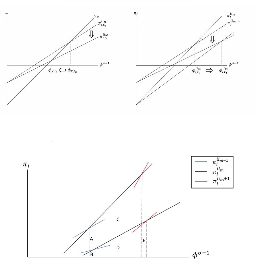
Figure 5: Predicted Impacts of Increasing Local Rebate Burden

Panel A. Changes in Exporting Technologies

(a) Direct exporting (b) Indirect exporting

Panel B. Interprovincial Trade Flow of Indirect Exports

Note: Panel A illustrates how the productivity cutoﬀs of direct and indirect exporting change if the share of the VAT

rebate burden to be paid by provincial governments increases. π

(φ) is the proﬁts of direct exporting of ﬁrm φ in

province i, and π

(φ) is the proﬁts of indirect exporting through province i

, the mth ranked province in province i’s

indirect exporting productivity cutoﬀ ladder (see Section 3.3 for detail). φ

is the productivity cutoﬀ of direct exporting

and φ

is the productivity cutoﬀ of indirect exporting from province i through i

. In (a), the cutoﬀ of direct exporting

shifts to the left as ﬁrms around the old cutoﬀ ﬁnd it more proﬁtable to switch to direct exporting. In (b), the cutoﬀ of

indirect exporting through province i

shifts to the right as ﬁrms around the old cutoﬀ ﬁnd it more proﬁtable to switch

to indirect exporting through province i

m−1

Panel B illustrates how the indirect export volume of province i through province i

would change given an increase in c.

The indirect export volume prior to the change is proportional to the sum of area A, B, C and D and the indirect export

volume after the change is proportional to the sum of area D and E. The eﬀect of the increase in c can be decomposed

into two parts, the price eﬀect which is proportional to area A and C and the network eﬀect which is proportional to area

A and B minus E. In the scenario shown in the ﬁgure, the overall eﬀect of an increase in c can be roughly approximately

by the price eﬀect since the former outweighs the latter by a large margin.

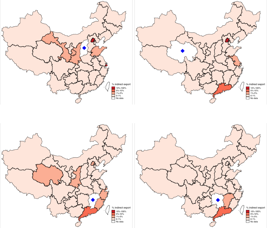
Figure 6: Heterogeneity in Reliance on Non-local FTCs for Indirect Exporting

(a) Shanxi (b) Qinghai

Note: This ﬁgures plots the baseline reliance on other provinces for indirect exporting in terms of the share of

indirect exports for four provinces, namely Shanxi, Qinghai, Jiangxi and Hunan. In each subﬁgure, the province

marked with a blue diamond is the manufacturing province that relies on other provinces for indirect exporting.

The ﬁgure exhibits clear heterogeneity among manufacturing provinces in terms of the degree of reliance on

each of other provinces for indirect exporting. The map is a map of land territory of China, which is based on

the standard map GS(2016)2884 from the Standard Map Service of the National Administration of Surveying,

Mapping, and Geoinformation of China.

Table 1: Summary Statistics of the Baseline Year

Variable Obs Mean SD Min Q1 Q2 Q3 Max

Panel A: FTCs (Customs Database)

Non-locally sourced FTC exports 11324 .844 4.08 0 0 .0109 .289 175

Locally sourced FTC exports 11324 5.52 17.5 0 .0968 .678 3.45 543

Share of locally sourced FTC exports 11324 .846 .276 0 .84 .993 1 1

Number of HS2 varieties 11324 12.6 13.3 1 2 7 19 67

Panel B: Manufacturing Firms (NBS Survey)

Is exporter prior to reform 57301 .249 .432 0 0 0 0 1

Indirect exports 57301 1.17 9.92 0 0 0 0 670

Direct exports 57301 .111 1.29 0 0 0 0 173

Total exports 57301 1.28 10.1 0 0 0 0 670

Average share of indirect exports 57301 .225 .405 0 0 0 0 1

Average share of indirect exports among exporters 14254 .903 .216 .00108 .971 1 1 1

Output 57301 .0944 .766 0 .011 .0225 .0525 86

Sales 57301 .0927 .759 0 .0107 .0219 .0512 86

Employment 57301 387 1852 0 76 150 312 126876

Is SOE 57301 .205 .404 0 0 0 0

Panel C: Industries (VAT Rebate Rate & NBS Survey)

VAT rebate rate (HS6) 5227 .137 .0373 0 .13 .15 .17 .17

Export intensity (HS2) 23 .245 .148 .0587 .122 .228 .288 .589

Panel D: Provinces (Provincial Statistical Yearbook)

GDP 31 45 37.4 1.85 23.9 28.6 60 158

Population 31 41.4 26.9 2.72 19.3 38.2 61.6 96.7

Fiscal revenue 31 3.83 3.55 .0982 1.67 2.66 4.07 15.8

Tax revenue 31 2.18 2.36 .0683 .847 1.27 2.12 9.87

Fiscal balance 31 .809 .83 -.0698 .31 .589 .887 4.08

VAT revenue 31 .697 .686 .0113 .278 .471 .734 2.82

Note: This table presents the summary statistics of the baseline year 2003 for the four main datasets we use in the analysis, namely the Chinese Customs

Database, the NBS Survey of Manufacturing Firms, the Export VAT Rebate Rate Database, and the Provincial Statistical Yearbooks. We organize the statistics

into four panels based on unit of observation: FTCs, manufacturing ﬁrms, industries, and provinces. In particular, Panel A is based on an unbalanced panel

of FTCs whereas Panels B, C, and D are all based on balanced panels. All summary statistics are in the baseline year 2003 except for average share of indirect

exports which is the 2001-2003 average and export intensity which is an industry’s average percentage of ﬁrms engaging in exporting activity in the NBS

survey between 2001 and 2003. The currency unit in Panel A and B is million USD and in Panel D is billion USD.

Table 2: Heterogeneity in Predicted Rebate Burden and Exposure Measure

Variable Obs Mean SD Min Q1 Q2 Q3 Max

Panel A: Provinces

Predicted rebate burden (amount) in 04 31 .00662 .00831 .000123 .00174 .00437 .00686 .0316

Predicted rebate burden (% ﬁscal revenue) in 04 31 .196 .163 .0379 .09 .161 .214 .86

Exposure measure in 04 31 .0187 .0168 .000565 .00971 .0134 .0214 .0744

Average non-locally sourced FTC exports 01-03 31 .212 .266 .00378 .0587 .14 .219 .99

% of non-locally sourced FTC exports 01-03 31 18.4 10.8 2.73 10.2 16.8 24.9 48.8

Average rebate rate of manufacturers in 04 31 .122 .00875 .102 .118 .126 .128 .13

Average rebate rate of FTCs in 04 31 .124 .0075 .104 .121 .127 .128 .132

Panel B: Province-industries

Exposure measure in 04 1977 .0237 .0529 1.72e-7 .00213 .00778 .0215 .86

Indirect exports in 03 1977 .0362 .142 0 .000345 .0026 .0168 2.01

Total exports in 03 1977 .0829 .298 0 .00106 .00779 .0418 4.22

Average rebate rate of manufacturers in 04 1977 .123 .0224 0 .127 .13 .13 .17

Note: This table presents the heterogeneity in 2004 predicted rebate burden and exposure measure and FTCs’ pre-reform sourcing pattern. The currency unit is billion

USD. In general, the 2004 predicted rebate amount is calculated as the pre-reform average of non-locally sourced FTC exports × the 2004 rebate rate × share of rebate

burden on provincial government (see Section 5.1 for details on constructing predicted burdens). We then scale it based on provincial governments’ ﬁscal capacity, namely

the pre-reform average of ﬁscal revenue. The exposure measure of a province is calculated as a weighted average of intermediary provinces’ predicted burden, weighted by

the reliance on each intermediary province (see Section 5.2 for details on constructing the exposure measure at both province and province-industry levels).

Table 3: Impact on Interprovincial Trade of Indirect Exports

Sample: China Customs Data 2001-2006,

Balanced Sample of Pairs of Manufacturing Province and Intermediary Province

Indirect exports from

manufacturing province

(1) (2)

from manufacturing province

(3) (4) (5) (6)

Predicted burden -6.181***

(1.115)

-5.888***

(1.110)

-0.0118***

(0.00311)

-0.0112***

(0.00308)

-11.35***

(2.738)

-6.856**

(3.109)

Observations 5580 5580 5580 5580 5580 5580

Pair FE Y Y Y Y Y Y

Year FE Y Y Y Y Y Y

Manufacturing province speciﬁc linear time trend Y Y Y Y Y Y

Intermediary province speciﬁc linear time trend Y Y Y Y Y Y

Manufacturing province weighted rebate rate Y Y Y

Intermediary province weighted rebate rate Y Y Y

Share of Indirect exports Number of FTCs hired

Note: This table examines the changes in interprovincial trade of export goods by intermediary provinces’ predicted rebate burden. Each observation is a pair of a

manufacturing province and an intermediary province in a given year. The dependent variables are indirect exports from the manufacturing province through FTCs in the

intermediary province (Columns 1 and 2), the value share of indirect exports through the intermediary province over all indirect exports from the manufacturing province

(Columns 3 and 4), and the number of FTCs in the intermediary province hired by the manufacturing province (Columns 5 and 6). We apply inverse hyperbolic sine

transformation on indirect exports to account for zero-valued observations. The key regressor of interests is the predicted rebate burden of the intermediary province (as %

of provincial ﬁscal revenue; see Section 5.1 for details on constructing predicted burdens). All regressions control for pair ﬁxed eﬀect, year ﬁxed eﬀect, intermediary-province-

and manufacturing-province-speciﬁc linear time trends. Even columns further control for the average rebate rate of the two provinces. Standard errors are clustered at the

province-pair level. *** implies signiﬁcance at 0.01 level, ** 0.5, * 0.1.

Table 4: Impact on FTCs’ Sourcing Activities

Sample: China

Customs Data 2001-2006, Unbalanced Sample of FTC

Non-locally

sourced

FTC exports

(1) (2)

Locally sourced

FTC exports

(3) (4)

Share of non-locally

sourced FTC exports

(5) (6)

Predicted burden -2.091***

(0.457)

-3.155***

(1.103)

-0.205

(0.314)

-1.282**

(0.568)

0.0925***

(0.0161)

0.105***

(0.0364)

Observations 100189 100189 100189 100189 100189 100189

Firm FE

Year FE

Province speciﬁc linear time trend

Province-level weighted rebate rate

Note: This table examines the changes in FTCs’ sourcing activities by local provinces’ predicted rebate burden. The dependent

variables are exports of an FTC bought from non-local manufacturers (Columns 1 and 2), exports of an FTC bought from local

manufacturers (Columns 3 and 4), and value share of exports from local manufacturers (Columns 5 and 6). We apply inverse

hyperbolic sine transformation on non-locally and locally sourced FTC exports to account for zero-valued observations. The regressor

of interest is the predicted rebate burden (as % of provincial ﬁscal revenue; see Section 5.1 for details on constructing predicted

burdens). All regressions control for ﬁrm ﬁxed eﬀect, year ﬁxed eﬀect, province-speciﬁc linear time trend. Standard errors are

clustered at the province level. *** implies signiﬁcance at 0.01 level, ** 0.5, * 0.1.

Table 5: Impact on Manufacturing Exports

Sample: China Customs Data 2001-2006, Balanced Sample of Chinese Province-industries

Indirect exports

(1) (2)

Total exports

(3) (4)

Exposure -6.73***

(1.52)

-6.75***

(1.51)

-9.23***

(1.94)

-9.23***

(1.93)

Observations 11862 11862 11862 11862

Province FE

Industry FE

Year FE

Province speciﬁc linear time trend

Weighted rebate rate

Note: This table examines the changes in manufacturing provinces’ exporting activities by exposure to reform. The dependent

variables are total exports produced in a manufacturing province-industry (Columns 1 and 2) and indirect export produced in a

province-industry (Columns 3 and 4). We apply inverse hyperbolic sine transformation on indirect exports and total exports to

account for zero-valued observations. The regressor of interest is the exposure measure constructed using the predicted burdens

(as % of provincial ﬁscal revenue; see Section 5.2 for details on constructing the exposure measures). The sample is a balanced

panel of province-industries from 2001 to 2006. All regressions control for province ﬁxed eﬀects, industry ﬁxed eﬀects, year ﬁxed

eﬀects, province-speciﬁc linear time trend, and weighted-rebate rate. Standard errors are clustered at the province level. ***

implies signiﬁcance at 0.01 level, ** 0.5, * 0.1.

Table 6: Impact on Manufacturing Firms

Sample:

China NBS Data 2001-2006, Balanced Sample of Baseline Exporters

Indirect exports

(1)

Direct exports

(2)

Total exports

(3)

Is indirect exporter

(4)

Is direct exporter

(5)

Panel A: Using exposure measure

IndirectDependence X Exposure -46***

(10.8)

18.4*

(9.81)

-46.2***

(11.6)

-2.66***

(.742)

3.42***

(.435)

Exposure 39.9***

(9.89)

-14.6

(9.24)

40.1***

(10.8)

2.3***

(.67)

-2.95***

(.288)

Observation 61206 61206 61206 61206 61206

Panel B: Using post-reform dummy

IndirectDependence X Post -2.6***

(.377)

1.25**

(.496)

-2.59***

(.378)

-.154***

(.0267)

.191***

(.00976)

Observation 61272 61272 61272 61272 61272

Firm FE

Year FE

Province speciﬁc linear time trend

Weighted rebate rate

Note: This table examines the changes in Chinese manufacturers’ production and exporting activities by its exposure to reform and reliance on indirect export

channel. The dependent variables are ﬁrms’ indirect exports, direct exports, total exports, and whether ﬁrms are indirect exporters or direct exporters. The sample

is a balanced panel of above-scale existing exporters prior to the reform. We apply inverse hyperbolic sine transformation on indirect exports, direct exports, and

total exports to account for zero-valued observations. The regressor of interest is the interaction term between the pre-reform dependence on indirect exporting

and either the exposure measure for Panel A (as % of provincial ﬁscal revenue; see Section 5.2 for details on constructing the exposure measures) or a post-reform

dummy for Panel B. The pre-reform dependence on indirect exporting is deﬁned as the pre-reform fraction of indirect exports over total exports. All regressions

control for ﬁrm ﬁxed eﬀects, year ﬁxed eﬀects, and province-speciﬁc linear time trend, and weighted-rebate rate. Panel A in addition controls for exposure. Standard

errors are clustered at the province level. *** implies signiﬁcance at 0.01 level, ** 0.5, * 0.1.

Table 7: Heterogeneous Impact on Manufacturing Firms by Ownership Type and Baseline Firm Size

Sample: China

NBS Data 2001-2006, Balanced Sample of Baseline Exporters

Indirect exp

orts

(1)

Direct exports

(2)

Total exports

(3)

Panel A: Heterogeneity on Firm Ownership

IndirectDependence X Exposure X SOE 59.6***

(14.4)

30.7

(19.2)

65.4***

(14.5)

IndirectDependence X Exposure -137***

(25.8)

-15.2

(22.9)

-146***

(27.2)

Exposure X SOE -60.6***

(14)

-38.3**

(18.3)

-66.1***

(14.3)

Exposure 133***

(24.7)

31.6

(21.1)

142***

(26.6)

Observation 29976 29976 29976

Panel B: Heterogeneity on Firm Size

IndirectDependence X Exposure X Pre-reform Output 3.52

(2.14)

.505

(3.75)

5.09**

(2.45)

IndirectDependence X Exposure -88.6***

(28.9)

13.9

(38.9)

-108***

(35.6)

Exposure X Pre-reform Output 3.52

(2.14)

.505

(3.75)

5.09**

(2.45)

Exposure 76.1**

(33.2)

-27.4

(43.2)

92.7**

(42.7)

Observation 61206 61206 61206

Firm FE

Year FE

Province speciﬁc linear time trend

Weighted rebate rate

Note: This table examines the heterogeneous eﬀect of the reform on Chinese manufacturers due to ownership types and baseline ﬁrm size.

The dependent variables are ﬁrms’ indirect exports, direct exports, and total exports. We apply inverse hyperbolic sine transformation

on indirect exports, direct exports, and total exports to account for zero-valued observations. The regressor of interest is the triple

interaction term between the pre-reform dependence on indirect exporting (deﬁned as the pre-reform fraction of indirect exports over

total exports), the exposure measure (as % of provincial ﬁscal revenue; see Section 5.2 for details on constructing the exposure measures),

and either a dummy indicating whether a manufacturer is SOE in Panel A or the baseline average output in Panel B. All regressions

control for ﬁrm ﬁxed eﬀects, year ﬁxed eﬀects, province-speciﬁc linear time trend, weighted-rebate rate, and other relevant interaction

terms in Equation 9. The sample is a balanced panel of above-scale manufacturers from 2001 to 2006. We further restrict the sample

in Panel A to either SOEs or private ﬁrms. SOE is deﬁned as ﬁrms whose state capital constitutes more than 50% of the total capital.

Standard errors are clustered at the province level. *** implies signiﬁcance at 0.01 level, ** 0.5, * 0.1.

Table 8: Robustness Check Using Non-Exporting Manufacturing Firms

Sample: China NBS

Data 2001-2006; Balanced Sample of Baseline Non-Exporters

Sales Output

(1) (2)

Exposure X Exp

ort Intensity above 75th Percentile -1.758*

(0.893)

-2.052**

(0.979)

Exposure X Export Intensity between 50th and 75th Percentile -0.035

(0.618)

-0.141

(0.542)

Exposure X Export Intensity between 25th and 50th Percentile -0.218

(0.630)

-0.295

(0.630)

Exposure 0.518

(0.469)

0.472

(0.441)

Observation 157411 157411

Firm FE

ear FE

Province speciﬁc linear time trend

Weighted rebate rate Y Y

Note: This table examines the diﬀerential eﬀect on manufacturers which do not have record of exporting in

the NBS survey prior to the reform. The dependent variables are sales and employment.We apply inverse

hyperbolic sine transformation on sales and output to account for zero-valued observations. The regressors

of interest are a set of double interaction terms between exposure measure (as % of provincial ﬁscal revenue;

see Section 5.2 for details on constructing the exposure measures) and dummies indicating whether the ﬁrm’s

industry is within a certain quarter of the distribution of export intensity. The sample is a balanced panel

of above-scale manufacturers which do not have record of exporting in the NBS survey prior to the reform.

All regressions control for ﬁrm ﬁxed eﬀects, year ﬁxed eﬀects, and province-speciﬁc linear time trend, and

weighted-rebate rate. Standard errors are clustered at the province level. *** implies signiﬁcance at 0.01

level, ** 0.5, * 0.1.

Table 9: Heterogeneous Impact on FTCs by Baseline Sourcing Activities

Sample:

China Customs Data 2001-2006, Unbalanced Sample of FTC-Industries

(1)

Dependent variable: FTC exports

(2) (3)

Predicted burden X 01-03 exports -1.111***

(0.182)

-1.112***

(0.179)

Predicted burden X 01-03 fraction

of rebate due to non-local exports

0.195

(0.496)

Predicted burden X 01-03 industrial

rebate rate

-2.46

(2)

Predicted burden 15.84***

(2.651)

15.79***

(2.719)

.139

(.325)

Observations 53076 53076 606061

Firm FE

Year FE

Province speciﬁc linear time trend

Province-level weighted rebate rate

Note: This table examines the heterogeneous eﬀect of the reform on FTCs’ exporting activities based on size and industry. The

observation is FTCs in Columns 1 and 2 and FTC-industry sub-ﬁrms in Column 3. The dependent variables are exports through

an FTC (-industry). We apply inverse hyperbolic sine transformation on FTC exports to account for zero-valued observations.

The regressors of interest are the interaction terms between province-level predicted rebate burden (as % of provincial ﬁscal

revenue; see Section 5.1 for details on constructing predicted burdens) and pre-reform export volume, average rebate rate of

non-locally sourced exports, and industrial average rebate rate respectively. All regressions control for ﬁrm ﬁxed eﬀect, year ﬁxed

eﬀect, province-speciﬁc linear time trend. Standard errors are clustered at the province level. *** implies signiﬁcance at 0.01

level, ** 0.5, * 0.1.

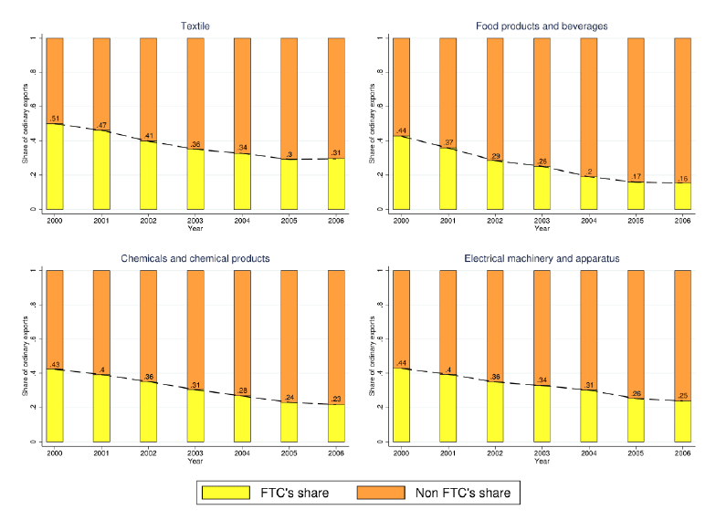
A Appendix Figures

Figure A.1: The Role of FTCs in Ordinary Exports: Four Export-intensive Industries

Note: This ﬁgure plots the share of exports via FTCs for four export-intensive industries, namely textile, food

products and beverages, chemicals and chemical products, and electrical machinery and apparatus.

Figure A.2: Number of Sourcing Locations of FTCs and direct exporters

Note: This ﬁgure plots the distribution of the number of sourcing locations of FTCs and direct exporters. FTCs

are classiﬁed using ﬁrm names following Manova and Zhang (2009)–see Section 4.2 for more detail.

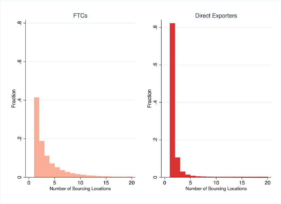
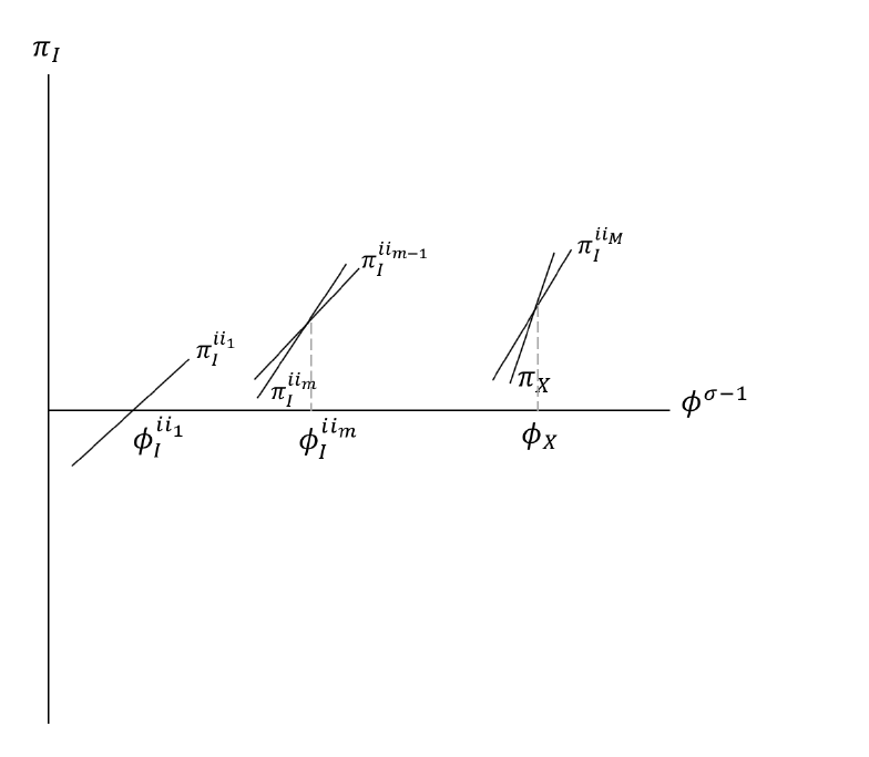
Figure A.3: The Productivity Cutoﬀs of Direct and Indirect Exporting Technologies

Note: This ﬁgure illustrates the productivity cutoﬀs of direct and indirect exporting technologies. π

(φ, j) is the

proﬁts of indirect exporting from province m

through m

(j), the jth ranked province in province m

’s indirect

exporting productivity cutoﬀ ladder (see Section 3.3 for detail). φ

is the productivity cutoﬀ of direct exporting

and φ

is the productivity cutoﬀ of indirect exporting from province m

through m

(j).

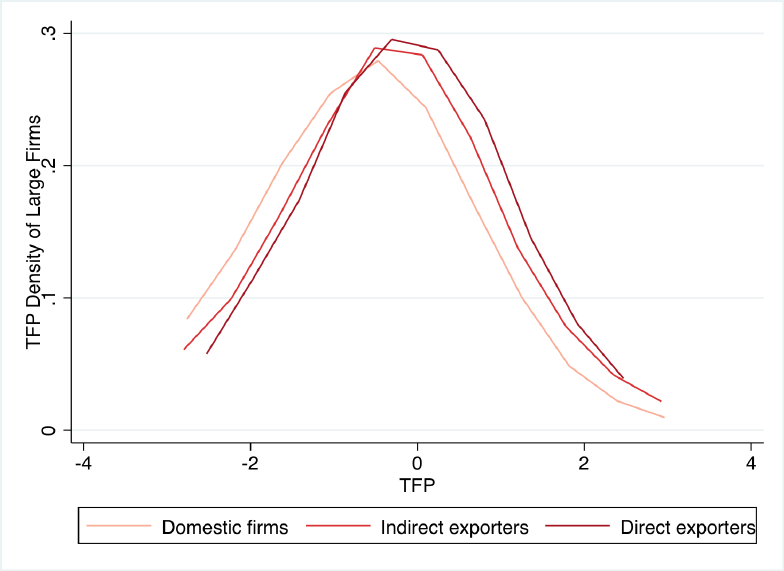
Figure A.4: The TFP Distribution of Diﬀerent Exporting Technologies

Note: This ﬁgure exhibits the probability distributions of TFPs of domestic ﬁrms and ﬁrms using diﬀerent

exporting technologies. The ﬁgure suggests that direct exporters are more productive than indirect exporters,

which are more productive than domestic ﬁrms.

B Appendix Tables

Table B.1: Sample Description of the NBS Survey of Manufacturing Firms (2001-2006)

Year Number of Firms % of Private Domestic Firms % of Exporting Firms

Panel A. Sample: All Industrial Firms in the Manufacturing Sector

2001 154278 0.32 0.26

2002 165815 0.39 0.27

2003 181131 0.47 0.28

2004 259302 0.54 0.3

2005 251434 0.57 0.3

2006 279205 0.6 0.28

Panel B. Sample: Balanced Panel from 2001-2006

2001 65453 0.34 0.35

2002 65453 0.37 0.36

2003 65453 0.39 0.37

2004 65453 0.41 0.39

2005 65453 0.42 0.38

2006 65453 0.43 0.38

Note: This table describes the sample of ﬁrms in the NBS Survey of Manufacturing

Firms. Panel A describes the full sample. Panel B describes the balanced sample from

2001 to 2006.

Table B.2: Heterogeneity Across Provinces in Predicted Rebate Burden and Exposure to Reform

Province 01-03 Avg FTC Export made Percentage of 01-03 Avg FTC Export 2004 Predicted 2004 Rebate burden 2004 Exposure Measure

by Non-local Manufacturers made by Non-local Manufacturers Rebate Amount as % Revenue (Revenue-Based)

Beijing 0.949 32.89 0.0286 0.45 0.0036

Tianjin 0.140 10.44 0.0044 0.20 0.0175

Hebei 0.099 8.19 0.0029 0.08 0.0201

Shanxi 0.060 10.20 0.0018 0.10 0.0629

Neimenggu 0.018 8.89 0.0005 0.04 0.0177

Liaoning 0.197 13.26 0.0059 0.12 0.0159

Jilin 0.035 15.26 0.0011 0.07 0.0214

Heilongjiang 0.088 28.79 0.0026 0.09 0.0220

Shanghai 0.919 11.64 0.0289 0.33 0.0006

Jiangsu 0.434 5.84 0.0136 0.17 0.0065

Zhejiang 0.333 2.73 0.0107 0.15 0.0134

Anhui 0.274 21.50 0.0088 0.36 0.0088

Fujian 0.175 4.53 0.0055 0.16 0.0322

Jiangxi 0.231 31.27 0.0073 0.41 0.0242

Shandong 0.219 6.31 0.0069 0.09 0.0125

Henan 0.101 19.70 0.0031 0.09 0.0162

Hubei 0.154 21.15 0.0050 0.17 0.0210

Hunan 0.186 20.77 0.0059 0.21 0.0167

Guangdong 0.990 10.37 0.0316 0.21 0.0125

Guangxi 0.116 23.35 0.0037 0.16

0.0275

Hainan 0.156 48.81 0.0049 0.86 0.0053

Chongqing 0.075 12.76 0.0024 0.15 0.0098

Sichuan 0.199 27.97 0.0063 0.18 0.0097

Guizhou 0.035 18.95 0.0010 0.08 0.0527

Yunnan 0.073 16.80 0.0023 0.09 0.0117

Xizang 0.004 34.20 0.0001 0.14 0.0021

Shan3xi 0.185 24.86 0.0058 0.31 0.0111

Gansu 0.059 20.74 0.0017 0.18 0.0057

Qinghai 0.023 35.69 0.0007 0.29 0.0744

Ningxia 0.007 7.38 0.0002 0.07 0.0117

Xinjiang 0.029 16.23 0.0009 0.07 0.0118

This table shows the heterogeneity across provinces in FTCs’ pre-reform inward-lookingness and the 2004 predicted rebate burden and exposure measure. The 2001-03 average

FTC export made by non-local manufacturers and the 2004 predicted rebate amount are denoted in billion USD. The 2004 predicted rebate amount is calculated as the pre-reform

average of the value of non-local exports of an industry ×the 2004 rebate rate of the industry×25%, which is then summing over all industries, where 25% is the share of VAT rebate

ﬁnanced by provincial governments. Finally, to calculate the rebate burden as % of the average pre-reform government revenue, we use information from the 2001-03 Provincial

Statistical Yearbook, where these values are reported in RMB and are converted to dollars using the exchange rate during 2001-03 (8.3 RMB ≈ 1 USD).

Table B.3: Correlation between Predicted Rebate Burden and Baseline Provincial Characteristics

(1) (2) (3) (4) (5) (6) (7)

Dependent variable: 2004 predicted burden

(8) (9) (10) (11) (12) (13) (14) (15) (16) (17) (18)

2003 provincial revenue .000026

(.0085)

-.28

(.3)

2003-04 growth in provincial revenue -.41

(.4)

-1.3

(.99)

2003 province balance -.0097

(.036)

.057

(.11)

2003-04 growth in provincial balance .0095

(.011)

.0072

(.026)

2003 provincial tax revenue .0043

(.013)

.41

(.37)

2003-04 growth in provincial tax -.18

(.28)

1.2

(.92)

2003 value-added tax -.012

(.044)

-.34

(.49)

2003-04 growth in value-added tax -.12

(.12)

-.32

(.59)

2003 provincial GDP -.00055

(.0008)

.0031

(.0088)

2003-04 growth in provincial GDP -.95

(.92)

-.64

(1.9)

2003 provincial population -.000015

(.000011)

.000027

(.000057)

2003-04 growth in provincial population 4.8

(3.3)

4.3

(8.3)

2003 total export -4.9e-13

(3.5e-12)

-5.4e-11

(1.4e-10)

2003 direct export -1.3e-12

(6.2e-12)

5.0e-11

(3.2e-10)

2003 indirect export -1.3e-12

(6.2e-12)

(.)

Number of FTCs .000015

(.000055)

-.000061

(.00045)

Number of exporters -1.5e-06

(8.5e-06)

.000082

(.0002)

Observation 31 31 31 31 31 31 31 31 31 31 31 31 31 31 31 31 31 31

Note: This table presents the regression coeﬃcients of 2004 predicted burden on the baseline provincial characteristics that may correlate with the outcome variables in Section 5.3.1 and 5.3.2. Columns 1 to 17 are

regressions on each single provincial characteristics and Column 18 is the regression on all provincial characteristics. The results show that the 2004 predicted burden are uncorrelated with any baseline provincial

characteristics.

Table B.4: Correlation between Exposure Measure and Baseline Provincial Characteristics

(1) (2) (3) (4) (5) (6) (7)

Dependent variable: 2004 exposure measure

(8) (9) (10) (11) (12) (13) (14) (15) (16) (17) (18)

2003 provincial revenue -.0014

(.00084)

-.028

(.031)

2003-04 growth in provincial revenue .0046

(.042)

-.14

(.1)

2003 province balance -.0024

(.0037)

.006

(.012)

2003-04 growth in provincial balance -.00095

(.0011)

-.0022

(.0028)

2003 provincial tax revenue -.0022*

(.0013)

.024

(.039)

2003-04 growth in provincial tax .041

(.028)

.13

(.097)

2003 value-added tax -.0064

(.0044)

.049

(.052)

2003-04 growth in value-added tax .02

(.012)

.0089

(.063)

2003 provincial GDP -.00011

(.000081)

-.0002

(.00093)

2003-04 growth in provincial GDP .031

(.097)

.05

(.2)

2003 provincial population -7.1e-07

(1.2e-06)

3.8e-06

(6.0e-06)

2003-04 growth in provincial population -.34

(.35)

.33

(.87)

2003 total export -3.8e-13

(3.5e-13)

8.5e-12

(1.4e-11)

2003 direct export -7.2e-13

(6.2e-13)

-2.6e-11

(3.3e-11)

2003 indirect export -7.2e-13

(6.2e-13)

(.)

Number of FTCs -6.5e-06

(5.6e-06)

-.000011

(.000048)

Number of exporters -1.1e-06

(8.6e-07)

.000018

(.000021)

Observation 31 31 31 31 31 31 31 31 31 31 31 31 31 31 31 31 31 31

Note: This table presents the regression coeﬃcients of 2004 exposure measure on the baseline provincial characteristics that may correlate with the outcome variables in Section 5.3.3 and 5.3.4. Columns 1 to 17 are regressions

on each single provincial characteristics and Column 18 is the regression on all provincial characteristics. The results show that the 2004 predicted burden are uncorrelated with any baseline provincial characteristics.

Table B.5: Impact on Interprovincial Trade of Indirect Exports: Alternative Measures of Rebate Burden

Sample: China Customs Data 2001-2006, Balanced Sample of Pairs of Manufacturing Province and Intermediary Province

Indirect exports from

manufacturing province

(1) (2)

Share of Indirect exports

from manufacturing province

(3) (4)

Number of FTCs hired

(5) (6)

Panel A: Province-pair level

Predicted burden (%tax) -2.762***

(0.536)

-2.637***

(0.534)

-0.00395***

(0.000958)

-0.00370***

(0.000942)

-3.670***

(1.215)

-1.795

(1.531)

Predicted burden (%balance) -0.394***

(0.0806)

-0.374***

(0.0786)

-0.000890**

(0.000449)

-0.000849*

(0.000448)

-1.045**

(0.446)

-0.749*

(0.451)

Predicted burden (%VAT) -0.644***

(0.104)

-0.613***

(0.104)

-0.00110***

(0.000333)

-0.00104***

(0.000322)

-0.964***

(0.265)

-0.490

(0.323)

Observations 5580 5580 5580 5580 5580 5580

Pair FE

Year FE

Manufacturing province speciﬁc linear time trend

Intermediary province speciﬁc linear time trend

Manufacturing province weighted rebate rate

Intermediary province weighted rebate rate

Panel B: Province-pair-industry level

Predicted burden (\%rev) -2.049***

(0.282)

-2.054***

(0.282)

-0.0212***

(0.00652)

-0.0212***

(0.00653)

-0.193

(0.235)

-0.199

(0.234)

Predicted burden (\%tax) -0.958***

(0.138)

-0.961***

(0.138)

-0.00633**

(0.00314)

-0.00632**

(0.00314)

0.0413

(0.162)

0.0381

(0.161)

Predicted burden (\%balance) -0.154***

(0.0265)

-0.154***

(0.0265)

-0.00159**

(0.000713)

-0.00159**

(0.000713)

-0.0240

(0.0255)

-0.0241

(0.0255)

Predicted burden (\%VAT) -0.197***

(0.0303)

-0.198***

(0.0303)

-0.00170**

(0.000691)

-0.00170**

(0.000691)

-0.00490

(0.0274)

-0.00548

(0.0273)

Observations 404052 404052 404052 404052 404052 404052

Pair FE

Year FE

Industry FE

Manufacturing province speciﬁc linear time trend

Intermediary province speciﬁc linear time trend

Manufacturing province-industry weighted rebate rate

Intermediary province-industry weighted rebate rate

Note: This table examines the changes in interprovincial trade of export goods by intermediary provinces’ predicted rebate burden. Each coeﬃcient in the table represents a

separate regression. Dependent variables are at province-pair-year level in Panel A and at province-pair-industry-year level in Panel B. The dependent variables are indirect

exports from the manufacturing province (-industry) through FTCs in the intermediary province, the value share of indirect exports through the intermediary province over

all indirect exports from the manufacturing province (-industry), and the number of FTCs in the intermediary province hired by the manufacturing province (-industry). We

apply inverse hyperbolic sine transformation on indirect exports to account for zero-valued observations. The key regressors of interests are various measures of predicted

rebate burden of the intermediary province. In separate regressions we use predicted burdens scaled by diﬀerent measures of local governments’ ﬁscal capacity (as % of

tax revenue, VAT revenue, and rollover balance respectively; see Section 5.1 for details on constructing predicted burdens) to test the robustness of the main results. All

regressions control for pair ﬁxed eﬀect, year ﬁxed eﬀect, intermediary-province- and manufacturing-province-speciﬁc linear time trends. Even columns further control for the

average rebate rate of the two provinces. The regressions in Panel B additionally control for industry ﬁxed eﬀects. Standard errors are clustered at the province-pair level.

*** implies signiﬁcance at 0.01 level, ** 0.5, * 0.1.

Table B.6: Impact on Interprovincial Trade of Indirect Exports: Two Consecutive Policy Reforms

Sample: China Customs Data 2001-2006, Balanced Sample of Pairs of Manufacturing Province and Intermediary Province

Indirect exports from

manufacturing province

(1) (2)

Share of Indirect exports

from manufacturing province

(3) (4)

Number of FTCs hired

(5) (6)

Predicted burden -1.264

(0.897)

-0.948

(0.889)

-0.00328**

(0.00150)

-0.00265*

(0.00150)

-3.105

(2.090)

1.408

(2.048)

Observations 5580 5580 5580 5580 5580 5580

Pair FE Y Y

Y Y Y Y

Year FE Y Y Y Y Y Y

Manufacturing province speciﬁc linear time trend Y Y Y Y Y Y

Intermediary province speciﬁc linear time trend Y Y Y Y Y Y

Manufacturing province weighted rebate rate Y Y Y

Intermediary province weighted rebate rate Y Y Y

Note: This table examines the changes in inte-rprovincial trade of export goods by the intermediary provinces’ predicted rebate burdens. Each observations is a pair of

a manufacturing province and an intermediary province in a certain year. The dependent variables are indirect exports from the manufacturing province through FTCs

in the intermediary province (Columns 1 and 2), the value share of indirect exports through the intermediary province over all indirect exports from the manufacturing

province (Columns 3 and 4), and the number of FTCs in the intermediary province hired by the manufacturing province (Columns 5 and 6). We apply inverse hyperbolic

sine transformation on indirect exports to account for zero-valued observations. The regressor of interests is the predicted rebate burden of the intermediary province (as

% of provincial ﬁscal revenue; see Section 5.1 for details on constructing predicted burdens). The predicted burden takes into account the adjustments of sharing rules

in both 2004 and 2005 (see Section about the two consecutive adjustments). All regressions control for pair ﬁxed eﬀect, year ﬁxed eﬀect, intermediary-province- and

manufacturing-province-speciﬁc linear time trends. Standard errors are clustered at the province-pair level. *** implies signiﬁcance at 0.01 level, ** 0.5, * 0.1.

Table B.7: Impact on FTCs’ Sourcing Activities: Alternative Measures of Rebate Burden

Sample: China Customs Data 2001-2006, Unbalanced Sample of FTC

Non-locally sourced

FTC exports

(1) (2)

Locally sourced

FTC exports

(3) (4)

Share of non-locally

sourced FTC exports

(5) (6)

Predicted burden (%tax) -1.175***

(0.327)

-1.459*

(0.776)

-0.122

(0.158)

-0.651*

(0.330)

0.0536***

(0.0120)

0.0518**

(0.0216)

Predicted burden (%balance) -0.0993***

(0.0242)

-0.0760***

(0.0230)

0.0126

(0.0129)

0.00850

(0.0149)

0.00513***

(0.000530)

0.00384***

(0.000479)

Predicted burden (%VAT) -0.267***

(0.0934)

-0.251

(0.162)

-0.0300

(0.0396)

-0.117

(0.0715)

0.0125***

(0.00367)

0.00961*

(0.00472)

Observations 100189 100189 100189 100189 100189 100189

Firm FE

Year FE

Province speciﬁc linear time trend

Province-level weighted rebate rate

Note: This table examines the changes in FTCs’ export activities by local provinces’ predicted rebate burden. Each coeﬃcient in the table

represents a separate regression. The dependent variables are exports of an FTC bought from non-local manufacturers (Columns 1 and 2),

exports of an FTC bought from local manufacturers (Columns 3 and 4), and value share of exports from local manufacturers (Columns 5 and

6). We apply inverse hyperbolic sine transformation on non-locally and locally sourced FTC exports to account for zero-valued observations.

The regressor of interests are various measures of predicted rebate burden. In separate regressions we use predicted burdens scaled by

diﬀerent measures of local governments’ ﬁscal capacity (as % of tax revenue, VAT revenue, and rollover balance respectively; see Section 5.1

for details on constructing predicted burdens) to test the robustness of the main results. All regressions control for ﬁrm ﬁxed eﬀect, year

ﬁxed eﬀect, province-speciﬁc linear time trend. Standard errors are clustered at the province level. *** implies signiﬁcance at 0.01 level, **

0.5, * 0.1.

Table B.8: Impact on FTCs’ Sourcing Activities: Two Consecutive Policy Reforms

Sample: China Customs Data 2001-2006, Unbalanced Sample of FTC

Non-locally sourced

FTC exports

(1) (2)

Locally sourced

FTC exports

(3) (4)

Share of non-locally

sourced FTC exports

(5) (6)

Predicted burden -1.833***

(0.289)

-2.103***

(0.523)

-0.984***

(0.330)

-1.986***

(0.465)

0.0259*

(0.0135)

-0.0191

(0.0134)

Observations 100189 100189 100189 100189 100189 100189

Firm FE

Year FE

Province speciﬁc linear time trend

Province-level weighted rebate rate

Note: This table examines the changes in FTCs’ export activities by local provinces’ predicted rebate burdens. The dependent variables are

exports of an FTC bought from non-local manufacturers (Columns 1 and 2), exports of an FTC bought from local manufacturers (Columns

3 and 4), and value share of exports from local manufacturers (Columns 5 and 6). We apply inverse hyperbolic sine transformation on

non-locally and locally sourced FTC exports to account for zero-valued observations. The regressor of interests is the predicted rebate

burden of the intermediary province (as % of provincial ﬁscal revenue; see Section 5.1 for details on constructing predicted burdens).

The predicted burden takes into account the adjustments of sharing rules in both 2004 and 2005 (see Section about the two consecutive

adjustments). All regressions control for ﬁrm ﬁxed eﬀect, year ﬁxed eﬀect, province-speciﬁc linear time trend. Standard errors are

clustered at the province level. *** implies signiﬁcance at 0.01 level, ** 0.5, * 0.1.

Table B.9: Impact on Manufacturing Exports: Alternative Measures of Exposure Measure

Sample: China Customs Data 2001-2006, Balanced Sample of Chinese Province-Industries

Indirect exports

(1) (2)

Total exports

(3) (4)

Exposure (%tax) -4.5***

(.992)

-4.52***

(.986)

-6.1***

(1.35)

-6.1***

(1.34)

Exposure (%balance) -.196*

(.1)

-.199*

(.102)

-.275*

(.15)

-.275*

(.15)

Exposure (%VAT) -.739***

(.219)

-.741***

(.218)

-.966***

(.263)

-.966***

(.262)

Observations 11862 11862 11862 11862

Province FE

Industry FE

Year FE

Province speciﬁc linear time trend

Weighted rebate rate

Note: This table examines the changes in manufacturing provinces’ exporting activities by exposure to reform. Each coeﬃcient

in the table represents a separate regression. The dependent variables are total exports produced in a manufacturing province-

industry (Columns 1 and 2) and indirect exports produced in a province-industry (Columns 3 and 4). We apply inverse hyperbolic

sine transformation on indirect exports and total exports to account for zero-valued observations. The regressors of interest are

various exposure measures. In separate regressions we use exposure measures constructed using diﬀerent predicted burdens

(as % of tax revenue, VAT revenue, and rollover balance respectively; see Section 5.2 for details on constructing the exposure

measures) to test the robustness of the main results. The sample is a balanced panels of province-industries from 2001 to 2006.

All regressions control for province ﬁxed eﬀects, year ﬁxed eﬀects, industry ﬁxed eﬀects, province-speciﬁc linear time trend, and

weighted-rebate rate. Standard errors are clustered at the province level. *** implies signiﬁcance at 0.01 level, ** 0.5, * 0.1.

Table B.10: Impact on Manufacturing Exports: Two Consecutive Policy Reforms

Sample: China Customs Data 2001-2006, Balanced Sample of Manufacturing

Province-Industries

Indirect exports

(1) (2)

Total exports

(3) (4)

Exposure -7.94***

(2.06)

-7.94***

(2.05)

-10.8***

(2.63)

-10.8***

(2.62)

Observations 11862 11862 11862 11862

Province FE

Industry FE

Year FE

Province speciﬁc linear time trend

Weighted rebate rate

Note: This table examines the heterogeneous eﬀect of the reform on Chinese manufacturers due

to ownership types and baseline ﬁrm size. Dependent variables are ﬁrms’ indirect exports, direct

expors, and total exports. We apply inverse hyperbolic sine transformation on indirect exports,

direct exports, and total exports to account for zero-valued observations. The regressor of interest

is the triple interaction term between the pre-reform dependence on indirect exporting (deﬁned as

the pre-reform fraction of indirect exports over total exports), a post-reform dummy, and either a

dummy indicating whether a manufacturer is SOE in Panel A or the baseline average output in

Panel B. All regressions control for ﬁrm ﬁxed eﬀects, year ﬁxed eﬀects, province-speciﬁc linear time

trend, weighted-rebate rate, and other relevant interaction terms in Equation (9). The sample is a

balanced panel of above-scale manufacturers from 2001 to 2006. We further restrict the sample in

Panel A to either SOEs or private ﬁrms. SOE is deﬁned as ﬁrms whose state capital constitutes

more than 50% of the total capital. Standard errors are clustered at the province level. *** implies

signiﬁcance at 0.01 level, ** 0.5, * 0.1.

Table B.11: Impact on Manufacturing Firms: Alternative Measures of Exposure Measure

Sample: China NBS Data 2001-2006, Balanced Sample of Baseline Exporters

Indirect exports

(1)

Direct exports

(2)

Total exports

(3)

Is indirect exporter

(4)

Is direct exporter

(5)

IndirectDependence X Exposure (%tax) -28.483***

(6.527)

11.125*

(6.222)

-28.563***

(7.045)

-1.642***

(0.455)

2.151***

(0.238)

Exposure (%tax) 24.921***

(5.979)

-8.584

(5.942)

25.045***

(6.557)

1.436***

(0.410)

-1.821***

(0.162)

IndirectDependence X Exposure (%balance) -4.958***

(0.969)

1.940**

(0.753)

-5.048***

(1.041)

-0.295***

(0.064)

0.329***

(0.055)

Exposure (%balance) 4.283***

(0.933)

-1.649**

(0.657)

4.372***

(1.018)

0.250***

(0.060)

-0.298***

(0.040)

IndirectDependence X Exposure (%VAT) -6.290***

(1.602)

2.472

(1.506)

-6.275***

(1.720)

-0.358***

(0.111)

0.480***

(0.065)

Exposure (%VAT) 5.522***

(1.446)

-2.014

(1.423)

5.506***

(1.572)

0.315***

(0.099)

-0.413***

(0.049)

Observation 61206 61206 61206 61206 61206

Firm FE

Year FE

Province speciﬁc linear time trend

Weighted rebate rate

Note: This table examines the changes in Chinese manufacturers’ production and exporting activities by its exposure to reform and reliance on indirect export channel. Each

coeﬃcient in the table represents a separate regression. The dependent variables are ﬁrms’ indirect exports, direct exports, total exports, and whether ﬁrms are indirect exporters

or direct exporters. We apply inverse hyperbolic sine transformation on indirect exports, direct exports, and total exports to account for zero-valued observations. The regressor

of interest is the interaction term between the pre-reform level of dependence on indirect exporting and the exposure measure. In separate regressions we use exposure measures

constructed using diﬀerent predicted burdens (as % of tax revenue, VAT revenue, and rollover balance respectively; see Section 5.2 for details on constructing the exposure

measures) to test the robustness of the main results. The pre-reform level of dependence on indirect exporting is deﬁned as the pre-reform fraction of indirect exports over total

exports. The sample is a balanced panel of above-scale existing exporters prior to the reform. All regressions control for ﬁrm ﬁxed eﬀects, year ﬁxed eﬀects, and province-speciﬁc

linear time trend, weighted-rebate rate and exposure. Standard errors are clustered at the province level. *** implies signiﬁcance at 0.01 level, ** 0.5, * 0.1.

Table B.12: Impact on Non-Exporters

Sample: China NBS Data 2001-2006, Balanced Sample of Baseline Non-Exporters

Indirect exports

(1)

Direct exports

(2)

Total exports

(3)

Is indirect exporter

(4)

Is direct exporter

(5)

Exposure -0.127

(0.458)

0.013

(0.123)

-0.137

(0.460)

-0.023

(0.032)

0.002

(0.009)

Observation 157411 157411 157411 157411 157411

Firm FE

Year FE

Province speciﬁc linear time trend

Weighted rebate rate

Note: This table examines the changes in Chinese manufacturers’ production and exporting activities by its exposure to reform and reliance on indirect export

channel. The sample is a balanced panel of above-scale non-exporters prior to the reform. The dependent variables are ﬁrms’ indirect exports, direct exports, total

exports, and whether ﬁrms are indirect exporters or direct exporters. We apply inverse hyperbolic sine transformation on indirect exports, direct exports, and total

exports to account for zero-valued observations. The regressor of interest is the exposure measure (as % of provincial ﬁscal revenue; see Section 5.2 for details on

constructing the exposure measures). All regressions control for ﬁrm ﬁxed eﬀects, year ﬁxed eﬀects, and province-speciﬁc linear time trend, and weighted-rebate

rate. Standard errors are clustered at the province level. *** implies signiﬁcance at 0.01 level, ** 0.5, * 0.1.

Table B.13: Heterogeneous Impact on Manufacturing Firms by Ownership Type and Baseline Firm Size

Sample: China NBS Data 2001-2006, Balanced Sample of Baseline Exporters

Indirect exports

(1)

Direct exports

(2)

Total exports

(3)

Panel A: Heterogeneity on Firm Ownership

IndirectDependence X Post X SOE 1.87***

(.67)

2.65***

(.803)

2.17***

(.67)

IndirectDependence X Post -3.27***

(.326)

1***

(.22)

-3.4***

(.32)

Post X SOE -2.03***

(.662)

-3.1***

(.828)

-2.31***

(.649)

Observation 30036 30036 30036

Panel B: Heterogeneity on Firm Size

IndirectDependence X Post X Pre-reform Output .102

(.121)

.342

(.275)

.192**

(.0796)

IndirectDependence X Post -3.62**

(1.37)

-2.63

(2.83)

-4.66***

(.919)

Post X Pre-reform Output .0546

(.0668)

-.193

(.284)

-.0171

(.0788)

Observation 61272 61272 61272

Firm FE

Year FE

Province speciﬁc linear time trend

Weighted rebate rate

Note: This table examines the heterogeneous eﬀect of the reform on Chinese manufacturers due to ownership types and baseline

ﬁrm size. Dependent variables are ﬁrms’ indirect exports, direct expors, and total exports. We apply inverse hyperbolic sine

transformation on indirect exports, direct exports, and total exports to account for zero-valued observations. The regressor of

interest is the triple interaction term between the pre-reform dependence on indirect exporting (deﬁned as the pre-reform fraction

of indirect exports over total exports), a post-reform dummy, and either a dummy indicating whether a manufacturer is SOE in

Panel A or the baseline average output in Panel B. All regressions control for ﬁrm ﬁxed eﬀects, year ﬁxed eﬀects, province-speciﬁc

linear time trend, weighted-rebate rate, and other relevant interaction terms in Equation (9). The sample is a balanced panel

of above-scale existing exporters prior to the reform. We further restrict the sample in Panel A to either SOEs or private ﬁrms.

SOE is deﬁned as ﬁrms whose state capital constitutes more than 50% of the total capital. Standard errors are clustered at the

province level. *** implies signiﬁcance at 0.01 level, ** 0.5, * 0.1.

C Mathematical Proofs

Prediction 1. For each province, the number and export volume of direct exporters weakly increases

in c.

Proof. Suppose after the increase in c province i

is still economically viable. Since f > f

∀m <

I I

M, province i

is still the highest in the indirect export productivity cutoﬀ ranking of province i.

Therefore, we have

z}|{

z }| {

 

z}|{

)

1−σ

∂φ

1 − (γ

= A ×

− f

∂c 1 − σ

≥0

z }| { z }| {

)

−σ

dγ

− f

(1 − (γ

)

1−σ

)

(σ − 1)(γ

) +

I I I

dc dc

− f

)

≤ 0

us, as c increases the productivity cutoﬀ of direct export shifts to the left, implying more manu-

facturers would export directly. On the other hand, if province i

is no longer an economically viable

option because of the increase in variable cost, then either a province down the productivity cutoﬀ

ranking or a previously economically unviable province would replace i

as the highest in the ranking.

It can be easily shown that the resulting productivity cutoﬀ of direct export would be smaller than

even before the reform. As a result, the number of direct exporters increases in c. The exporting

 

1−σ

revenue of direct exporter φ is r

(φ) = R

which does not change with c, so province i’s total

ρφP

direct export volume

∞

= r

(φ)dG(φ)

(12)

increases in c as the range of integration expands with c.

Here we relax the assumption that the local province of ﬁrm φ is ranked the lowest in the indirect

export productivity cutoﬀ ladder, i.e. i = i

, and prove a more general version of Prediction 2:

Prediction 2

. For each province, the number of its indirect exporters weakly decreases in c. Further-

dγ

�

/dc



I I

more, the export volume of its indirect exporters also weakly decreases in c if

dγ

∀m, n s.t. γ

/dc

Proof. Suppose after the increase in c province i

is still economically viable and therefore the lowest

in the productivity cutoﬀ ranking.

z}|{





{

∂φ

z}|{

)

1−σ

(γ

I I

= A ×

∂c 1 − σ

≤0

z }| { z }| {

dγ

(1 − σ)(γ

)

−σ

(γ

)

1−σ

−

I I I

dc dc

)

≥ 0

us, the productivity cutoﬀ of indirectly exporting from the most easily accessed FTC province

weakly increases in c. On the other hand, if province i

is no longer an economically viable option

because of the increase in variable cost, then either a province up the productivity cutoﬀ ranking or a

previously economically unviable province would replace i

as the lowest in the ranking. It can be easily

shown that the resulting lowest productivity cutoﬀ of indirect exporting would be larger than φ

even

before the reform, leading to the same result as above. Combining with the proof of Prediction 1 we

can see that the range of productivity of indirect export [φ

, φ

] shrinks as c increases.

dγ

�

I I

/dc



I I

Now we show that, given

dγ

∀m, n s.t. γ

< γ

, the volume of indirect export

I I

/dc

from province i decreases as well. To do so, we demonstrate that the volume of indirect export from any

existing indirect exporters of province i decreases in c. First, we show that, if the set of economically

viable provinces (and therefore the productivity cutoﬀ ranking) does not change, then all such provinces

∂φ

become less accessible after the reform, i.e.

≥ 0 ∀m ∈ [1, M]. We have proven this for m = 1. For

∂c

m ≥ 2,

{

z }| {



(γ

j−1



∂φ

z}|{

)

1−σ

− (γ )

1−σ

I I I

= A ×

∂c 1 − σ

− f

m−1

I I

z }| {

dγ

m−1

z }| {

�

dγ



(γ

)

−σ

m−1

)

−σ

m−1

(1 − σ) − (γ − f )

I I I I

dc dc

−

m−1

− f )

I I

z }| {

�

m−1



((γ

)

1−σ

− (γ

m−1

)

1−σ

)

I I

−

I I

dc dc

m−1

− f )

I I

> 0

(13)

(14)

∂

(φ) ∂

(φ)

which is a direct result from the inequality condition that implies

σ−1 σ−1

< 0 if γ

∂φ ∂c ∂φ ∂c

. This means that, after the reform, ﬁrms used to indirectly export through province i

m−1

would

ﬁnd it even more challenging to move up to i

which had a higher ﬁxed cost but a lower variable

∂φ

Even though we prove that

> 0, without further assumptions we do not know about the relative magnitudes of

∂c

the derivatives for diﬀerent m.

cost of indirect exporting, since marginal proﬁt of exporting through province i

would decrease more

substantially. The increasing barrier to entry thus drives the productivity cutoﬀ of province i

to the

right.

Given the results above, a ﬁrm which used to export indirectly through province i

would ﬁnd itself

in either of the four following situations after the reform:

1. continue to export through i

;

2. export through some province lower than i

in the pre-reform productivity cutoﬀ ranking;

3. export through some province used to be economically unviable;

4. exit the foreign market.

In ﬁrst three cases the ﬁrm would face a higher variable cost of indirect exporting unless it continues

to export through its local province, and in the last case the ﬁrm would stop exporting all together.

Therefore, a ﬁrm’s indirect export will always weakly decrease in c regardless of its productivity. Since

the number of indirect exporters of province i also decreases in c, its volume of indirect export decreases

in c.

Prediction 3. Given an increase in c, for any province i:

1. the local exporters rely more on local intermediary after the reform, i.e. the number and export

volume of i’s indirect exporters through local intermediary (which is i

) increase in c;

2. the export volume of i’s indirect exporters through province i

, m ∈ [2, M − 1] decreases if the

price eﬀect outweighs the network eﬀect;

3. the number and export volume of m’s indirect exporters through province i

decreases.

Proof. Since own province has the lowest ﬁxed cost, the own province is ranked at the last in the produc-

dγ

tivity cutoﬀ ladder, i.e., i = i. By Assumption 1

= 0. We can therefore observe from inequality

∂φ

(13) that

= 0. From inequality (14) we also know that

> 0. Therefore, as c increases the

∂c ∂c

range of productivity that chooses to indirectly export from province i expands. As for the eﬀect on

, by Assumption 1 the price eﬀect is zero. Since Θ(φ) is an

increasing function of φ, the network

eﬀect is positive. Thus, the indirect export volume through province i’s own intermediary increases.

As for province i

, m ∈ [2, M − 1], the price eﬀect is strictly negative by Assumption 1. If in

addition the price eﬀect dominates the network eﬀect, the overall eﬀect of c on R

follows the sign

the price eﬀect. In this case, as c increases, province i’s indirect export volume through each of such

provinces decreases.

For province M, the price eﬀect is also strictly negative. Moreover, the network eﬀect is also strictly

negative, since we have proved by inequality (12) that φ

is a decreasing function of c and by inequality

(14) that φ

is an increasing

function of c. These together imply that the number and export volume

of province i’s indirect exporters through i

decrease as c increases.

Prediction 4. If the price eﬀects are suﬃciently larger than the network eﬀects, given an increase in

c a province will experience larger percentage decrease in indirect export through provinces from which

higher cost shocks are generated.

∂γ

∂R

/∂c /∂c /∂c /∂c

I I I I

Proof. We want to prove that if

then

. Suppose the price eﬀects

I I I I

m+1

∂R

∂r (φ)

are suﬃciently larger than the network eﬀects such that ≈ dG(φ), we only need to

∂c

show that the price eﬀect as a percentage of indirect export volume when exporting through province

is larger than that when through province i

. The price eﬀect through i

Z Z



∂r

dγ



1−σ

(φ)

dG(φ) = (1 − σ)(γ

)

−σ

RdG(φ)

∂c dc ρφP

 

1−σ

dγ

/dc τγ

I I

= (1 − σ) RdG(φ)

ρφP

dγ

/dc

= (1 − σ)

dγ

/dc

The price eﬀect relative to export volume through i

is therefore (1 − σ)

. Similarly, the

relative

dγ /dc

price eﬀect through i

is (1 − σ)

, and percentage decrease in indirect exporting through

will be higher

∂γ /∂c ∂γ /∂c

than that through i

I I

as long as

I I

Prediction 5. Suppose the price eﬀects are suﬃciently larger than the network eﬀects. Given a

marginal increase in c, a province with higher exposure will experience a larger percentage decrease in

export volume of indirect exporters.

Proof. The indirect exporting volume from province i is

= .

Following Equation (1), if the price eﬀects are suﬃciently larger than the network eﬀects, the per-

centage change in indirect exporting volume w.r.t. a marginal increase in c is approximately

∂R

/∂c

I I

∂c

m+1

∂r

(φ)

≈ dG(φ)

∂c

∂γ

/∂c

= (1 − σ)

= (1 − σ)E

(15)

where the second to third step follows from Equation (15). Thus, if province i has higher exposure than

∂R /∂c

province j, we can easily see from above that